UNIVERSIDADE TÉCNICA DE LISBOA
INSTITUTO SUPERIOR DE ECONOMIA E GESTÃO
MESTRADO EM: Economia Monetária e Financeira
MONETARY POLICY IN A CURRENCY UNION WITH
HETEROGENEOUS COUNTRIES
CARLA SOFIA CAEIRO SOARES
Orientação: Doutor João Miguel Sousa
Júri:
Presidente: Doutor Luís F. Costa
Vogais: Doutor João Miguel Sousa
MONETARY POLICY IN A CURRENCY UNION WITH HETEROGENEOUS COUNTRIES
Carla Sofia Caeiro Soares
M.Sc.: Monetary and Financial Economics
Supervisor: João Miguel Sousa
Viva Voce Exam in:
ABSTRACT
We build a two-country DSGE model for a currency union, with habit formation,
product and labour differentiation and nominal rigidities. Monetary policy is defined by a
rule that responds to the area’s macro-variables averages weighted by each country's size.
We intend to study the impact of different sources of heterogeneity between the countries
(home bias in consumer preferences, wage and price mark-ups and wage and price setting
rigidity) on both countries and the union. The model is calibrated and the response to
shocks is simulated. The main innovation is the incorporation of several sources of
heterogeneity and the assessment of its impact on welfare.
The main results of the model simulation are the following: (i) only heterogeneity
regarding the home bias can lead to differentials in consumer price inflation; (ii)
heterogeneity regarding wage or price mark-ups does not lead to significantly different
responses to shocks of the countries; (iii) heterogeneity on nominal rigidities results in
differences among the countries’ response, favouring the more flexible country and
resulting in smoother and longer impacts when shocks occur in the more rigid country.
We also examine the volatility of the variables and perform a formal utility-based
welfare analysis. We find out that nominal rigidities are the most important source of
heterogeneity. In a currency union where the central bank responds to the area wide and
does not take into account national differences, it is preferable to increase flexibility in
both countries and in both wages and prices, as there are significant welfare losses when
countries attempt to make only wages or prices more flexible, or when only a single
country is flexible. A comparison of different policy rules allows us to conclude that
simpler rules (without interest rate smoothing) provide the best result in terms of welfare.
Keywords: DSGE models, currency union, monetary policy rules, heterogeneous
POLÍTICA MONETÁRIA NUMA UNIÃO MONETÁRIA COM PAÍSES HETEROGÉNEOS
Carla Sofia Caeiro Soares
Mestrado em: Economia Monetária e Financeira
Orientador: João Miguel Sousa
Provas concluídas em:
RESUMO
É desenvolvido um modelo DSGE de dois países que formam uma união
monetária, com hábitos no consumo, diferenciação de bens e de trabalho e rigidez
nominal. A política monetária segue uma regra que responde à média das variáveis macro
do agregado, ponderada pela dimensão do país. Pretende-se estudar o impacto de
diferentes fontes de heterogeneidade entre os países (preferências no consumo enviesadas
a favor de bens nacionais, mark-ups dos salários e preços e rigidez nos salários e preços) em ambos os países e na união. O modelo é calibrado e são simuladas as respostas a
choques. A principal inovação consiste na incorporação de várias fontes de
heterogeneidade e na avaliação do impacte em termos de bem-estar.
As simulações do modelo levam aos principais resultados: (i) apenas a
heterogeneidade no enviesamento das preferências do consumo provoca diferenciais na
inflação no consumidor; (ii) heterogeneidade nos mark-ups de preços e salários não resulta em respostas significativamente diferentes entre os países; (iii) heterogeneidade no grau
de rigidez nominal implica diferentes respostas dos países, favorecendo o país mais
flexível e levando a respostas mais suaves e prolongadas quando os choques ocorrem no
país mais rígido.
Também se analisa a volatilidade das variáveis e o bem-estar de acordo com uma
função formal derivada a partir da função utilidade. Conclui-se que a rigidez nominal é a
fonte de heterogeneidade mais relevante. Numa união monetária onde o banco central
responde à união e não considera as especificidades de cada país, é preferível aumentar a
flexibilidade em ambos os países e nos preços e salários simultaneamente, dado que
flexibilizar só salários ou preços, ou se só um país for flexível, leva a elevadas perdas de
bem-estar. Conclui-se ainda que regras de política monetária simples (sem gradualismo da
taxa de juro) promovem o melhor resultado de bem-estar.
Palavras-chave: modelos DSGE, união monetária, regras de política monetária, países
AGRADECIMENTOS
No final desta etapa, tenho que dirigir agradecimentos às pessoas que
contribuíram, directa ou indirectamente, para o desenvolvimento deste trabalho.
Em primeiro lugar, tenho muito que agradecer ao meu orientador, Doutor João
Miguel Sousa, por todo o apoio técnico e pessoal, pelas sugestões, esclarecimentos,
conselhos e disponibilidade.
Quero também expressar o meu agradecimento ao Banco de Portugal,
nomeadamente à direcção do Departamento de Mercados e Gestão de Reservas, por ter
facilitado a frequência do mestrado; aos colegas e coordenadores da Área de Operações de
Política Monetária deste departamento, pelo todo o apoio prestado ao longo desta fase e
pela ajuda à frequência da parte lectiva; à Área de Política Monetária do Departamento de
Estudos Económicos, nomeadamente ao coordenador da área, pelo apoio especial na fase
final da dissertação.
O meu agradecimento dirige-se também a aquelas pessoas que se disponibilizaram
para ler e comentar este trabalho, nomeadamente ao Doutor Luís Costa e ao Doutor
Bernardino Adão.
Ainda do ponto de vista técnico, devo o meu agradecimento a Vítor Saraiva, por
me ter dado a conhecer a desigualdade de Hölder.
Finalmente, tenho a agradecer o apoio e ajuda dos meus pais, que ao longo das
suas vidas têm lutado para que eu aproveite oportunidades que a eles nunca foram dadas.
Last, but not the least, um grande reconhecimento e agradecimento a Henrique Monteiro, cuja companhia e apoio nestes últimos anos foram essenciais para este trabalho, para
ultrapassar as fases difíceis, para encontrar o tempo e a motivação para continuar, e
Contents
1 Introduction 4
2 Brief summary of literature 7
3 Description of the model 14
3.1 Households and consumption . . . 16
3.2 Labour supply and wages . . . 20
3.3 Firms . . . 23
3.4 Market equilibrium . . . 28
3.5 Area wide economy . . . 30
3.6 The log-linearized model . . . 30
4 Simulation and analysis of the results 34 4.1 Homogeneous countries and common shocks . . . 35
4.1.1 Calibration . . . 35
4.1.2 Model dynamics . . . 38
4.2 Heterogeneous countries . . . 42
4.2.1 Model dynamics . . . 43
4.2.2 Different monetary policy rules . . . 49
4.2.3 Welfare analysis . . . 57
5 Conclusions 68
A Appendix - The steady-state model 71
B Appendix - Equations for the foreign economy in the log-linearized
model 72
D Appendix - Determination of the welfare function 80
D.1 Approximation of the utility from consumption . . . 80
D.2 Approximation of the disutility from working . . . 81
D.2.1 Approximation of the wage dispersion measure . . . 83
D.2.2 Approximation of aggregate labour and price dispersion measure . . 85
D.3 Welfare expression . . . 89
E References 91
List of Figures
1 Schematic representation of the model . . . 15
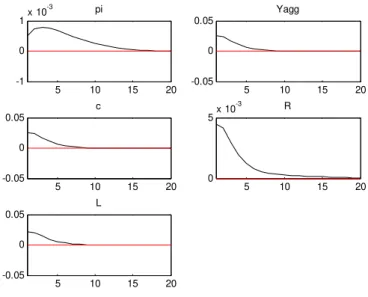
2 Area wide variables’ impulse responses to a common preference shock (ξbt). 38
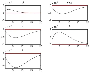
3 Area wide variables’ impulse responses to a common labour supply shock
(ξLt). . . 39
4 Area wide variables’ impulse responses to a common productivity shock
(ηa,t). . . 40
5 Area wide variales’ impulse responses to a common monetary policy shock
(ξmt ). . . 41
6 Area wide variables’ volatility considering different monetary policy rules and different parameter values. . . 54 7 Home economy variables’ volatility considering different monetary policy
rules and different parameter values. . . 55 8 Foreign economy variables’ volatility considering different monetary policy
rules and different parameter values. . . 56 9 Welfare analysis considering different policy rules and different parameter
10 Area wide welfare log-deviations from the steady-state for different degrees
of nominal rigidity, maintaining countries equal at all times. . . 65
11 Welfare analysis for different degrees of nominal rigidity of the home econ-omy, while the foreign remains unchanged. . . 66
12 I.r.f. when countries are homogeneous. . . 74
13 I.r.f. when the home country differs on the home bias ( ). . . 75
14 I.r.f. when the home country differs on the wage mark-up (ϕ). . . 76
15 I.r.f. when the home country differs on the wage rigidity (ξDw). . . 77
16 I.r.f. when the home country differs on the price mark-up (θ). . . 78
1 Introduction
Since 1999, thirteen European countries have abandoned their national currencies and
autonomous monetary policy in favour of the European Monetary Union (EMU). This
can be considered as a "live experience" of the Optimal Currency Areas (OCA) theory
and has motivated numerous studies on this area of research. According to this theory,
it is more advantageous for various regions to share the same currency together when
there is a sufficient level of synchronization and integration of trade and labour markets among the regions, i.e., when regions are similar enough. Despite the increased economic
integration between European countries, namely regarding trade and financial markets,
there are member countries which show persistent differentials against the euro area, namely regarding inflation and output growth. For instance, Greece, Spain and Ireland
have been persistently growing above the euro area average since the mid-1990’s, while
Germany and Italy have remained below the average (Benalal et al., 2006). As for inflation
differentials, Greece, Spain, Ireland, the Netherlands and Portugal have showed persistent positive inflation differentials while Germany, France and Austria have been situated in the opposite group (ECB, 2003). These differentials can be explained by an ongoing convergence process, but there may also exist structural differences among countries, such as different features in goods, labour or capital markets that justify diverging economic dynamics among countries.
On the other hand, the monetary policy of the euro area is defined according to the
euro area as a whole. The Governing Council of the European Central Bank (ECB) has
as the main objective to stabilize prices, so that inflation, measured by the Harmonized
Index of Consumer Prices (HICP), remains in the medium term at a level below but close
to 2%.
In this paper, we are interested in understanding the implications of having
wide and for each member country. The model is quite general and can be applied to any
currency area, although we try to approach it sometimes in the study to the euro area.
Several sources of heterogeneity are considered: (i) differences in consumer preferences regarding the country where the goods are produced (home bias), since it is acceptable
for consumers in the European Union to prefer to consume national goods; (ii) diff er-ences in wages and prices mark-up, as labour and product markets in euro area countries
can diverge in their institutional features; and (iii) differences in wage and price setting mechanisms, as there are studies that point out the existence of different levels of nominal and real rigidity (Dhyne et al., 2005; Dickens et al., 2006, among others). In this way,
our main innovation in comparison to the current literature is the incorporation of more
sources of heterogeneity, particularly an interaction between wage and price rigidity, and
the assessment of its impact on welfare, through the assessment of variables’ volatility
and through the use of a quadratic approximate welfare measure (Benigno and Woodford,
2004). This analysis is developed under the framework of a two-country Dynamic
Stochas-tic General Equilibrium (DSGE) model, including habit formation, product and labour
differentiation, monopolistic competition and nominal rigidities. This type of models is currently more frequently used for monetary policy analysis, given that these models seem
to be able to replicate well the behaviour of main macroeconomic variables in response to
a wide set of shocks (Smets and Wouters, 2003).
The model is calibrated and the impact of shocks1, both common and country-speci
fic,
is simulated. We find that the source of heterogeneity that leads to the most significant
differences between countries’ impulse response functions is the nominal rigidity, both on wages and prices. Differences in the home bias are relevant because they are the only source of heterogeneity responsible for differences in consumer price inflation, in a context of perfectly free trade of goods among the area. Regarding the welfare analysis, we
obtain interesting results. First, nominal rigidities are the source of heterogeneity which
has the most important consequences on welfare. In a currency union where the central
bank responds to the aggregate and does not take into account national differences, it is preferable to increaseflexibility in both countries and in both wages and prices, as there
are significant overall welfare losses for both economies when countries attempt to make
only wages or prices moreflexible, or when only a single country isflexible. Second, we
find that simpler monetary policy rules seem to provide the best result in terms of welfare.
We abstract from fiscal policy issues, making the simplifying assumption that there
is no government. This assumption is made since we are more interested in assessing
the impacts of different sources of country heterogeneity in a currency union instead of the interactions between monetary and fiscal policy. Nonetheless, we acknowledge that
when fiscal policy is taken into account, the negative impacts of asymmetries between
countries or asymmetric shocks in a currency union are less relevant. Adão et al. (2006)
argue that in a currency union with price rigidities, asymmetric countries or shocks and
incomplete internationalfinancial markets,fiscal policy can offset the negative impacts of these aspects and lead to zero costs of a currency union, as long as labour is not mobile.
The paper is structured as follows. Section 2 provides the context on the theoretical
discussions where this study can be fit in. Section 3 presents and describes the model,
which will be calibrated and simulated in section 4. Under section 4, we have afirst
sub-section (4.1) on the special case of homogeneous countries in order to try to replicate the
euro area wide behaviour, while in a second subsection (4.2) the effects of heterogeneous countries are discussed. This discussion evolves in three parts: firstly, on the impacts
of shocks (subsection 4.2.1); secondly, on the volatility analysis comparing various policy
rules (subsection 4.2.2), and thirdly, on the consequences on welfare for each country and
for the aggregate of the various sources of heterogeneity and the various policy rules
2 Brief summary of literature
Currently, DSGE models are frequently used for monetary policy analysis. These are
mathematical models that incorporate microeconomic foundations, following a general
equilibrium methodology in a dynamic and stochastic environment. This type of models
evolved mainly from Real Business Cycle (RBC) models, which first appeared in the
1980s. RBC theory claimed thatfluctuations in overall economic activity were due to real
economic shocks, such as changes in the rate of technical progress. The RBC models were
relatively small general equilibrium models, micro-founded, and were able to replicate
some features regarding economic growth and fluctuations. However, the economies of
these models were usually subject to a technology shock and were characterized by price
flexibility and perfect competition. In this way, there was no role for monetary policy.
Monetary policy only could have temporary real effects and monetary policy disturbances had no real effect since agents were able to perfectly forecast its impact in aggregate nominal expenditure. However, empirical evidence does not seem to support this result.
Empirical studies, namely through the application of Vector Autoregressive (VAR)
methodology, suggest that, in the medium term, monetary policy has a temporary impact
on output and a more lasting impact on inflation. Results from VAR estimation differ according to the country studied, the period chosen or the monetary policy variables used.
However, two main conclusions can be drawn (Walsh, 2003):
1. Output follows a hump-shaped pattern in response to a monetary policy shock,
before slowly returning to the baseline scenario and the effects of the shock have faded out. The maximum effect on output generally occurs after a relatively long lag of around 2 years.
2. A "price puzzle" arises, as an increase in the interest rate leads to an increase in
possi-ble explanation to this puzzle is that central banks usually have more information
than the rest of the agents and therefore anticipate the necessary monetary policy
decisions, since they are aware of its "long and variable lags" before it takes effects.
In the 1990s, another type of models appeared which extended the RBC methodology
and introduced nominal price and/or wage rigidity, maintaining the optimizing behaviour
of agents and micro-foundations. These models are build up in a dynamic, stochastic,
general equilibrium framework. This theory is also called the New-Keynesian synthesis,
as it includes Keynesian features as market imperfections build up in a general equilibrium
framework. Some reference papers of DSGE models with applications to monetary
pol-icy analysis are Clarida et al. (1999), McCallum and Nelson (1999), Smets and Wouters
(2003). Galí (2002) overviews the main features and advantages to monetary policy
analy-sis that DSGE models allow. These models usually share the following common features:
nominal rigidity on prices and/or wages, usually with a price setting mechanism à la Calvo;
monopolistic competition and product differentiation and monetary policy is usually rep-resented by a rule for the nominal interest rate. These characteristics lead to models
that can be broadly summarized in three parts: (i) the demand side is represented by
an IS curve with expectations, (ii) the supply side is represent by a Phillips curve, which
presents inflation with forward looking components and (iii) a policy rule for the interest
rate,ad-hoc or optimized from the central bank’s objective function.
DSGE models permit to consider a wide set of economic disturbances (Christiano et
al., 2005; Smets and Wouters, 2003). Frequently, these models are estimated for a country
or currency area, which make them quite useful for central bankers (Smets and Wouters,
2003). The possibility of having a structural interpretation for the movements in the data
given the inclusion of various shocks, is an advantage in comparison to the VAR analysis.
More recently, this type of models has also been used in forecasting, given the developments
(Smets and Wouters, 2004).
At the same time, the OCA theory was developed and "applied" in the euro area. A
region is an OCA when it is advantageous to its members to share a currency together
(Mundell, 1961). A group of regions will benefit from sharing a currency together if
(i) shocks hitting the regions are not asymmetric, (ii) there is a high degree of labour
mobility and/or wageflexibility and (iii) there is a centralizedfiscal authority responsible
for the redistribution of resources among the regions. When countries share a currency
together, they give up their autonomous monetary policy and, therefore, one of the means
to respond to shocks. If shocks hit the member countries in the same way, monetary policy
response will be the right one for all countries. However, when shocks are asymmetric,
the best monetary policy reaction would differ from country to country and they lack the policy adjustment mechanism. The second and third conditions work as the adjustment
mechanisms of countries in a currency area when subject to asymmetric shocks: labour
could move from one country to another or wages could differ between countries in order to reestablish the equilibrium; otherwise, the government could make transfers to the
member countries adversely impacted by the shock.
There is a connection between economic integration and economic specialization and
the costs and benefits of countries sharing the same currency. The greater the
special-ization of a country according to its comparative advantages, the more likely it would
be hit by asymmetric shocks, which would increase the costs of an OCA. When economic
integration increases, the intra-industry trade increases, decreasing the likelihood of
asym-metric shocks and, therefore, increasing the benefits of an OCA as countries have economic
efficiency gains from this linkage. Frankel and Rose’s (1997) empirical study shows that economic integration favours business cycle synchronization, which increases the benefits
of forming a currency union. Then, according to these authors, the European Union could
In this way, from the process of european economic integration resulted that the Treaty
establishing the European Community defined the Statutes of the European System of
Central Banks (ESCB), despite several authors not considering the euro area as an OCA.
The primary objective of the ESCB is to attain price stability; without prejudice to this
objective, the ESCB shall promote the Community policies aiming at promoting growth
and employment. When the Governing Council of the ECB decides on monetary policy,
it bases its decisions on developments in euro area as a whole.
Issing et al. (2001) summarizes the features of the euro area economy. Member
countries share a similar industrial structure, have a significant weight of the public sector
in Gross Domestic Product (GDP) and share a similar financial structure based on the
banking system. On the other hand, there are significant economic imbalances among
countries and regions of the euro area, with quite different levels of income per capita. Besides, countries have different institutional features regarding labour markets and the euro area as a whole is closer to the rest of the world than each individual member.
There are empirical studies showing that euro area countries are not homogenous.
According to Benalal et al. (2006), the GDP growth dispersion among euro area countries
remains fairly stable, with some countries systematically above or below the euro area’s
average. These differences seem to reflect structural differences among countries, as the business cycle synchronization has increased, which favours Frankel and Rose’s (1997)
thesis. Inflation also differs among countries, as we observe persistent inflation differentials in the euro area. These inflation differentials are due to some non-structural factors (differences in profit margin and unit labour cost developments, in administered price and indirect tax changes and in cyclical positions), but also to structural factors, such as the
impact of nominal convergence effects triggered by EMU, structural rigidities and, to a limited extent, income convergence and Balassa-Samuelson effects (ECB, 2003).
price and wage setting, which is one of the sources of heterogeneity considered in our
model, seems to be different across euro area countries. Dhyne et al. (2005) find that heterogeneity in price setting behaviour across countries is relevant, although partially
related to differences in the consumption structure. This also suggests that there is also heterogeneity regarding consumer preferences, another source of heterogeneity considered
in our model. Differences among countries seem to be more significant and pronounced regarding wage rigidity. Dickens et al. (2006) find that there are substantial differences across countries2, namely in the degree of downwards real and nominal wage rigidity.
This type of cross-country asymmetries has implications on the effects of monetary pol-icy. Recently, literature has been studying the effects of heterogeneity among the regions of a currency union using DSGE models for more than one country. Usually, two-country
models are developed, with the usual features: product differentiation, monopolistic com-petition, nominal rigidities and completefinancial markets. The countries in the models
are open to each other while closed to the rest of the world. Monetary policy also follows
what happens in the euro area, with a common central bank setting the interest rate
according to a rule which usually is a function of the currency area’s average inflation and
output. Then, some distinct aspects between countries are introduced.
Benigno (2004) builds a two-region model with product differentiation between regions, monopolistic competition, price rigidity and labour immobility between regions. Regions
are subject to asymmetric shocks. He also defines a welfare criterion in order to evaluate
monetary policy in the currency area. It is found that the optimal monetary policy should
lead to a high degree of inflation inertia. When the monetary policy authority responds to
the average of the area, weighted by the regions size, the optimal is not attained. But the
optimal plan can be approximated by an inflation targeting policy which gives a higher
weight to the inflation in the region where nominal rigidities are more striking.
Gomes (2004) studies the implications for a currency area of different price rigidity degrees in response to common and specific shocks by using a calibrated model. The
degree of price rigidity differs between countries. Shocks, either common or specific, lead to significant differentials between countries, which are larger when shocks are idiosyn-cratic. These differentials are favourable to the less sluggish country. When the more rigid country is hit by the shock, impacts are smoother, mainly in the other country. She
also compares different monetary policy rules. Rules that result in the best outcome for aggregate variables do not mean that they also lead to the best individual result. Interest
rate smoothing stabilizes inflation and output, reduces countries differentials, but it also reduces inflation correlation between countries. A rule which responds to the output gap
diminishes output volatility with prejudice for inflation volatility and decreases output
volatility in the more rigid country while increasing it in the other, reducing, therefore,
output correlation between the countries.
Other contributions focus more on labour market specificities. Abbritti (2007) studies
how countries in a currency union with different institutional features regarding labour markets respond to shocks, either common or specific, in a calibrated model. In his
model, there is also rigidity in real wages (Hall’s wage norm) and there is no migration
between countries. The real wage rigidity increases the persistence of temporary shocks
and contributes to explain the lasting inflation and unemployment differentials. Addition-ally, more sclerotic labour markets increase inflation volatility and reduce unemployment
volatility. The author also finds that common (monetary policy) shocks can also have
large asymmetric effects. Finally, strict inflation targeting is found not to be optimal, as it leads to large and persistent unemployment fluctuations, either at the aggregate or
individual levels.
There is another line of investigation more focused on estimation of these type of
Thefirst of these papers develops a model with habit formation, price rigidity à la Calvo,
product differentiation and home bias in consumption goods. It also allows for different preferences and technologies between countries, although with labour as the only input
in production. They then estimate the model for some European countries (Germany,
France and Italy) and analyze the costs, in terms of welfare, of ignoring the member
countries’ heterogeneity. Theyfind out that in the case of an optimal monetary policy
based on the area wide model, then there are relatively larger welfare losses than when the
optimal rule is derived from the multi-country model. Then, the central bank should take
into consideration the specific features of the countries forming the currency area, both
in terms of behavioral parameters and specific shocks, as the welfare losses are due to the
use of a sub-optimal forecasting model, instead of the use of a policy rule which responds
to the aggregate variables. Additionally, they alsofind out that introducing interest rate
smoothing in the welfare function does not change significantly the results.
Pytlarczyk’s (2005) estimated model for Germany and the remaining euro area seems
to allow a consistent analysis of the interaction between these two regions. This model is
slightly more evolved than Jondeau and Sahuc (2006), as it includes some features present
in Smets and Wouters (2003) such as capital and an adjustment cost of capital, price and
wage rigidity à la Calvo, product and labour differentiation and external habit formation. The model presented in our paper follows the line of research of the above mentioned
papers, and goes beyond them by mixing some features as wage and price rigidity and home
bias in consumer preferences with the purpose of comparing different ad-hoc monetary policy rules in terms of their impact in each country and in the main aggregate variables
and welfare. In this way, the main innovation of this paper refers to the combined analysis
of price and wage rigidity in heterogeneous countries, showing the impacts on welfare
from changing theflexibility of price and wage setting mechanisms. We also consider the
in labour and goods markets (through differences in wage and price mark-ups), although these sources of heterogeneity have a smaller impact on welfare. Finally, we consider the
impact of different monetary policy rules, all of which respond to the aggregate average variables, as it occurs in the euro area.
3 Description of the model
We build a currency union model consisting of two economies, the domestic economy
(variables denoted by D and parameters without an asterisk) and the foreign economy
(variables denoted by F and parameters with an asterisk). The two countries form together
a currency area, meaning that they share the same currency and have a common central
bank that implements monetary policy for the aggregate. The population of the aggregate
area is a continuum of identical and infinitely lived agents in the interval[0,1](aggregate
size is then normalized to 1), which produce a bundle of differentiated goods. Households are denoted by j. When these live in the domestic economy, we have j ∈ [0, n], while
when they live in the foreign economyj ∈(n,1]. Therefore, nis the relative size of the
home economy. Similarly, each firm produces one differentiated good i. Then, index i denotes bothfirms and goods. Relative output size of each economy corresponds to the
relative population size. When i ∈ [0, n], the firm belongs to the home economy and
wheni ∈(n,1], it belongs to the foreign economy. In order to easily identify where the
household orfirm belong to, whenever considered adequate, we will denote the household
orfirm belonging to the foreign country with an asterisk (j∗ ori∗).
All goods are tradable, there is free trade of goods andfinancial markets are complete.
However, labour markets are specific to each country, i.e., there is no mobility of labour
between the two countries. Figure 1 presents a schematic representation of the model.
The model follows closely DSGE models used recently in the literature. Indeed, we
Figure 1: Schematic representation of the model
Households D
L Aggregator
Continuum of differentiated goods
D homogeneous good
Households F
L Aggregator
Continuum of differentiated goods
F homogeneous good
MP authority
Differentiated labour Dixit-Stiglitz
aggregator Monop. competition Calvo wages
Homogeneous labour aggregate
Cobb-Douglas production function Monop. Competition Calvo Prices
Dixit-Stiglitz aggregator Perfect competition
Consumption home bias
Interest rate rule
Consumption home bias
Differentiated labour
Dixit-Stiglitz aggregator Monop. competition Calvo wages Homogeneous
labour aggregate
Cobb-Douglas production function Monop. Competition Calvo Prices
Dixit-Stiglitz aggregator Perfect competition
we simplify by excluding capital from our model. Adjustment between countries occurs
through the goods market, since labour is restricted to each country. The Smets and
Wouters (2003) model structure is applied to a two-country model, which brings it close
to Benigno (2004) and Jondeau and Sahuc (2006). These models assume optimal wage
setting, while in the model we develop here we introduce rigidity in wage setting. Evidence
from the euro area suggests that wages are rigid, specially downwards, and that wage
rigidity differs between countries (Dickens et al., 2006). Both prices and wages are set according to a Calvo mechanism with indexation to past inflation. Calvo price/wage
setting mechanism is the most commonly mean of introducing price/wage rigidity in the
recent literature. It is an useful feature as it can be solved without explicitly tracking
the distribution of prices acrossfirms and it is able to capture the factors that contribute
introduce costs of price adjustment (Rotemberg, 1982, 1996). Although the Rotemberg
sticky price model and the Calvo price model lead to a similar Phillips curve, they have
different implications for micro data: the Rotemberg model implies a single price in the micro data, while the Calvo model has implicit a distribution of prices among firms,
which seems to be more plausible. There are also models with staggered price setting
using Taylor contracts, which imply a certain time between price adjustments (Chari et
al., 2000), but can be criticized by not accounting for the sluggish response of inflation
adjustment. Regarding wage stickiness, wefind in the literature the introduction of Taylor
wage contracts, which will impact on price rigidity. Indeed, with these wage contracts,
prices display inertia but the inflation rate does not need to show inertia (Walsh, 2003).
3.1 Households and consumption
Households in each economy consume differentiated goods, either produced internally or imported. All households within each economy share the same preferences and
endow-ments but supply tofirms resident in the respective country differentiated labour. There is heterogeneity in households behaviour across countries. The representative household
jin both economies seeks to maximize its expected discounted utility, where the discount
factorβis common to the area wide:
E0 ∞
X
t=0
βtUt(j) (1)
The instantaneous utility function Ut(j) shares the same functional form for both
economies, depending positively on consumption ¡CD t , CtF
¢
and negatively on labour
¡
LD t , LFt
¢
; but it can differ in respect to the consumption habit ¡HD t , HtF
¢
, the
rela-tive risk aversion coefficients on consumption (σc, σ∗c)and on labour supply (σl, σ∗l)and
the preference¡εbD t , εbFt
¢
and labour supply¡εLD t , εLFt
¢
shocks.
economy andj∗ in the foreign one are, respectively:
UtD(j) = εbDt
∙ 1
1−σc
¡
CtD(j)−HtD¢1−σc− ε
LD t
1 +σl
LDt (j)1+σl
¸
(2)
UtF(j∗) = εbFt ∙
1 1−σ∗
c
¡
CtF(j∗)−HtF¢1−σ∗c
− εLFt
1 +σ∗
l
LFt (j∗)1+σ∗l
¸
Households present external habit formation, in the sense that their utility depends not
only on current consumption but also on how it differs from a proportion of the previous period total consumption in the respective economy: HD
t = hCtD−1 and HtF =h∗CtF−1,
where h(h∗) is the habit persistence parameter (in line with the "catching up with the
Joneses" argument presented in Abel, 1990). Following the recent literature (Smets and
Wouters, 2003; among others), including external habit persistence seems to provide a
greater correspondence to consumption behaviour, which seems to be more persistent
and to respond more gradually to economic shocks, as consumers dislike large and rapid
changes in consumption or can not change their consumption rapidly (especially if we
consider goods such as housing) (Fuhrer, 2000).
Consumers in both countries consume goods produced in either country. Thus, total
consumption in the home economy includes the consumption of internally produced goods
(CD,t) and imported goods (CF,t) from the foreign country. The consumption baskets of
the representative households in the home and foreign economies are given by (following
Jondeau and Sahuc, 2006):
CtD(j) = (CD,t(j)) (CF,t(j)) 1−
(1− )(1− ) (3)
CtF(j∗) = (CD,t(j
∗)) ∗(C
F,t(j∗))1−
∗
∗ ∗
(1− ∗)(1− ∗) (4)
In our model we include the hypothesis of the existence of home bias in preferences,
given by the parameterω (ω∗). In this way, ω(ω∗) is the share of domestically produced
ω = 0.5(ω∗ = 0.5), then consumers do not distinguish goods by the country were they
were produced. In caseω >0.5(ω∗>0.5), consumers prefer goods produced in the home
economy (CD,t), i.e., we have a home bias in consumption preferences. In case ω <0.5
(ω∗ <0.5), consumers prefer goods produced in the foreign economy (C
F,t).
CD,t(j)(CF,t(j)) is the consumption by householdjof domestically (foreign) produced
goods, which are imperfect substitutes and can either be consumed in the country where
they are produced in or can be exported and consumed by households in the other country.
In this way,CD,t(j)(CF,t(j)) is an index given by the following CES aggregator:
CD,t(j) =
"µ1
n
¶1
θZ n 0
CD,t(i, j)
θ−1
θ di
# θ θ−1
(5)
CF,t(j) =
"µ 1
1−n
¶1
θ∗Z 1
n
CF,t(i∗, j)
θ∗−1
θ∗ di∗
# θ∗ θ∗−1
CD,t(i, j) (CF,t(i∗, j)) is the consumption by household j of the generic goodi (i∗)
produced in the home (foreign) economy. Since goods produced in the same country
are differentiated, θ (θ∗) denotes the elasticity of substitution between goods produced in home (foreign) economy. These goods are then aggregated taking into account the
product differentiation and the production size of the country where they are produced.3
Households maximize their intertemporal utility function subject to an intertemporal
budget constraint which states that their income from labour, dividends and financial
markets applications will be fully used every period for consumption and transactions in
financial markets. The total income of each household is given by the labour income, where
wD,t (wF,t) denotes the real wage, and dividends from participating in the imperfectly
3Take also note of the following definitions, which will be useful for the market equilibrium conditions:
CD D,t=
n
0 CD,t(j)djas the total consumption of home produced goods in the home economy;
CF D,t=
1
nCD,t(j∗)dj∗as the total consumption of home produced goods in the foreign economy;
CD F,t=
n
0 CF,t(j)djas the total consumption of foreign produced goods in the home economy;
CF F,t=
1
competitive firms (DivD
t for households in D and DivtF for households in F), which are
denominated in units of the consumption basket of the respective country. Households
also receive income from the applications made in the bond market in the previous period.
Indeed, households can trade area wide riskless bonds Bt. These are one-period bonds
with price bt. Each domestic (foreign) household detains the same amount of Bt(j)
(Bt(j∗)). The bond market must be balanced in order to avoid the existence of Ponzi
games. Therefore, thefinancial market is at equilibrium at each moment when the area
aggregate is neither at a debtor nor at a creditor position (nBt(j) + (1−n)Bt(j∗) = 0).
The transversality condition holds and neither of the economies individually can assume a
permanent debtor or creditor position (lim
t→∞btnBt(j) = 0andtlim→∞bt(1−n)Bt(j
∗) = 0).
The income from applications in bonds made in the previous period and the transactions
made in the current period are defined in nominal terms. In order to make it consistent
with the remaining budget constraint, we have to divided it byPcD
t (PtcF), the consumer
price index for the home (foreign) economy.
Households also have access to a country-specific state-contingent securitySD t (StF),
denominated in units of the domestic (foreign) consumption basket. This security allows
an harmonization between households in the same country, so that all the households are
similar regarding consumption and area wide common asset holdings. Within each region,
there is a zero net supply of these state-contingent securities, i.e., R0nSD
t (j)dj = 0and
R1
nStF(j∗)dj∗= 0. In this way, we define the intertemporal budget constraint as follows
(for domestic households and for foreign households, respectively):
btBt(j)
PcD t
= Bt−1(j) PcD
t
+wD,t(j)LDt (j) +DivDt (j) +StD(j)−CtD(j) (6)
bt
Bt(j∗)
PcF t
= Bt−1(j∗) PcF
t
+wF,t(j∗)LtF(j∗) +DivtF(j∗) +StF(j∗)−CtF(j∗)
The optimization problem of the representative household in each economy resumes to
to the constraint (6), i.e., corresponds to the optimization of the following Lagrangian:
£=E0
∞ X t=0 βt ⎧ ⎪ ⎪ ⎨ ⎪ ⎪ ⎩ εbD t ∙ 1
1−σc
¡
CD
t (j)−HtD
¢1−σc
− ε LD t
1 +σl
LD t (j)
1+σl
¸
−
−λD,t
µ
btBt(j)−Bt−1(j) PcD
t −
wD,t(j)LDt (j)−DivtD(j)−StD(j) +CtD(j)
¶ ⎫ ⎪ ⎪ ⎬ ⎪ ⎪ ⎭
Thefirst-order conditions yield the usual Euler equation, i.e., the optimal consumption
flows over time, when we derive the Lagrangian with respect toBt(equation 7), and the
marginal utility from consumption when we derive the Lagrangian with respect to CD t
(equation 8), whereRt=
1 bt
is the gross nominal rate of return on bonds.
Et
∙
βλD,t+1 λD,t
RtPtcD
PcD t+1
¸
= 1 (7)
λD,t=εbDt
¡
CD t −HtD
¢−σc (8) Similar equations are found for the foreign economy.
3.2 Labour supply and wages
Households provide labour services to thefirms and the type of labour that each
house-hold provides is different from each other, so that households are competitive monopolist suppliers of differentiated labour. In other words, labour services provided by one house-hold are assumed byfirms to be different from the labour services provided by another household from the same country (Erceg et al., 2000). In this way, households sell their
labour services to firms and set their wages in each period in order to maximize their
utility given their budget constraint.
Labour markets are specific to each economy and there is no mobility of labour between
the home and the foreign economy. The way labour markets function in the two economies
following a Calvo mechanism. This means that not all households can adjust their wages
optimally on every period. A particular household can reoptimize its nominal wage only
when it receives a signal to do so. When optimizing the new wage, the household takes
into account the likelihood of being able to reoptimize its wage again in the future (Erceg
et al., 2000; Smets and Wouters, 2003). When the household does not receive this signal
to reoptimize, it adjusts wages as a function of past inflation.
The probability of a household in the home economy receiving the signal to optimize
its nominal wage toW˜D,t(j)is given by1−ξD
w. The rest of the households are not able
to reoptimize their wages (with probabilityξDw) and therefore can only adjust their wages
according to past inflation. Then, the wage is set as follows:
WD,t(j) =
⎧ ⎪ ⎪ ⎨ ⎪ ⎪ ⎩
˜
WD,t(j) with probability1−ξDw
µPcD t−1 PcD
t−2
¶γw
WD,t−1(j) with probabilityξDw
(9)
The parameter γw in equation (9) is the degree of wage indexation. When γw = 0
there is no indexation and the wages that can not be reoptimized remain constant; if
γw= 1, it implies perfect indexation to past consumer inflation.
Given labour differentiation, domesticfirms transform the differentiated labour services provided by domestic households into a labour indexLD
t that follows a Dixit-Stiglitz type
aggregator (Erceg et al., 2000):
LDt =
⎡ ⎣
µ
1 n
¶1
ϕZ n
0
¡
LDt (j)¢
ϕ−1
ϕ dj
⎤ ⎦
ϕ ϕ−1
(10)
LD
t (j)is the labour supplied by householdj. The parameterϕrepresents the elasticity
of substitution between different types of labour services within the home economy. The nominal wage index at home (WD,t) is also defined in a similar way:
WD,t=
∙1
n
Z n
0
(WD,t(j))1−ϕdi
¸ 1 1−ϕ
WD,t(j)denotes the nominal wage negotiated by householdj at datet. In this way,
householdjfaces the following labour specific demand from allfirms in the home economy:
LDt (j) =
µ
WD,t(j)
WD,t
¶−ϕLD t
n (12)
Households set their wages in order to optimize their intertemporal objective function
(1) subject to the budget constraint (6) and the above labor demand (12). The
optimiza-tion problem leads to the following mark-up equaoptimiza-tion for the optimized nominal wage
˜ WD,t4:
˜ WD,t PcD t Et ∞ X k=0 ³
βξDw´k ϕ−1 ϕ L˜
D t+kUC0D
t+k
Ã
PcD t+k−1 PcD
t−1
!γw
PcD t+k
PcD t
=−Et
∞
X
k=0
³
βξDw´kL˜D t+kUL0D
t+k (13)
Equation (13) states that the optimal wage will be set at the level where the
disu-tility from an additional working hour equals a mark-up over the increase in marginal
utility from consumption due to the higher working hours. The termsU0
CD
t+k and U 0
LD t+k
denote, respectively, the marginal utility from consumption and the marginal disutility
from labour5 andL˜D
t+k is the labour supplied at momentt+kby householdj which
reop-timized its wage at momentt, i.e., is the labour supply in time given that the household
was allowed to reoptimize its wage in the initial moment.
The law of motion of the home aggregate index of the nominal wage can be derived
from equations (9) and (11) is given by:
4Similarly to what happens in the price setting, the average optimal wage equation will be similar to the individual optimal wage. Although households provide differentiated labour and, therefore, face
different wages, they still share the same utility function and the same budget constraint and are not
subject to individual shocks. Thus, we can consider them as representative households in the sense that
the decision they take is the same and they will all choose the same wage (Erceg et. al, 2000; Woodford,
2003).
5Recall thatU0
CD t+k
=εbD
t+k(CDt+k(j)−HtD+k)−σc andUL0D t+k
=εbD
t+kεLDt+k LDt+k σL
(WD,t)1−ϕ=ξDw
"
WD,t−1
µ
PcD t−1 PcD
t−2
¶γw#1−ϕ
+³1−ξDw´ ³W˜D,t
´1−ϕ
(14)
We get similar expressions for the foreign economy. The wage indexation for the
households which can not reoptimize is WF,t(j∗) =
µPcF t−1 PcF
t−2
¶γ∗w
WF,t−1(j∗). The labour
demand in this country is given by LF t (j∗) =
µ
WF,t(j∗)
WF,t
¶−ϕ∗ LF t
1−n, while aggregate labour and aggregate wage are defined by the equations:
LF t = ⎡ ⎣ µ 1 1−n
¶ 1
ϕ∗Z 1
n
¡
LF t (j∗)
¢ϕ∗−1
ϕ∗ dj∗ ⎤ ⎦
ϕ∗
ϕ∗−1
WF,t =
∙
1 1−n
Z 1
n
(WF,t(j∗))1−ϕ
∗
dj∗
¸1−1ϕ∗
Taking the optimization problem similar to the home economy, i.e., the maximization
of the intertemporal utility function regarding wage subject to the budget constraint and
the labour demand equation, we reach a similar mark-up equation for the optimized wage
in the foreign country:
˜ WF,t
PF,tEt
∞
X
k=0
³
βξFw´k ϕ ∗−1
ϕ∗ L˜
F t+kUC0F
t+k
Ã
PcF t+k−1 PcF
t−1
!γ∗w
PtcF+k PcF
t
=−Et
∞
X
j=0
³
βξFw´kL˜Ft+kU0
LF t+k (15)
The law of motion of the foreign aggregate index of the nominal wage follows
(WF,t)1−ϕ
∗
=ξFw
"
WF,t−1
µPcF t−1 PcF
t−2
¶γ∗w#1−ϕ ∗
+³1−ξFw´ ³W˜F,t
´1−ϕ∗
(16)
3.3 Firms
There is a continuum of imperfectly competitive firms. Firms producing in the home
economy belong to the interval[0, n], whilefirms producing in the foreign country belong
behaviour according to the economy they belong to. This means that equations
summariz-ingfirms’ behaviour share the same functional form but with different parameters. Firms produce differentiated goods which are bundled into homogeneous domestic and foreign baskets of goods which can be freely traded among the area wide. The homogeneous
domestic and foreign goods (YD
t and YtF) are given by the following Dixit-Stiglitz type
aggregator, which takes into account households preferences (Erceg et al., 2000):
YtD=
"µ1
n
¶1
θ Z n 0
YtD(i)θ−θ1di
# θ θ−1
andYtF =
"µ 1
1−n
¶1
θ∗ Z 1
n
YtF(i∗)θ∗−θ∗1di∗
# θ∗ θ∗−1
(17)
The domestic firmi only produces one goodi, which is differentiated from the goods produced by other domesticfirms. Firms only have one productive factor, labour. In this
way, and for the home economy, the individual production function (YD
t (i)) depends on
labour (LD
t (i)), productivity (ADt ) andfixed costs (ΦD).6
YtD(i) =AtDLDt (i)−Φ D
n (18)
Productivity differs from economy to economy, but in both it is assumed to follow an AR(1) process: AD
t = (1−ρa) ¯AD+ρaADt−1+ηa,t, whereA¯Dis the long-term productivity,
ρais the persistence parameter andηa,tis a random shock.
Cost minimization conditions imply that the demand from all households for goods
produced byfirmi follows:
YtD(i) =
µ
PD,t(i)
PD,t
¶−θ
YD t
n (19)
where PD,t(i) is the price of good i and PD,t is the price index of home produced
6Following Christiano et al. (2005), fixed costs are included so that there is a minimum level of production that covers thefixed costs. Also in Christiano et al. (2005), it is argued thatfixed costs are
goods. Allfirms share the same marginal costs, given by the nominal wage weighted by
productivity:
M CtD=WD,t AD
t
(20)
Similarly to what was defined for wages, prices are also set by firms according to a
Calvo mechanism. At each periodt,firmiis allowed to reoptimize and chooses the price
˜
PD,t(i)with probability
³
1−ξDp´. If thefirm does not receive the signal to reoptimize (with probabilityξDp ), then it sets its price according to past inflation. In this way, price
is set according to
PD,t(i) =
⎧ ⎪ ⎪ ⎨ ⎪ ⎪ ⎩
˜
PD,t(i) with probability1−ξDp
µ
PD,t−1 PD,t−2
¶γp
PD,t−1(i) with probabilityξDp
(21)
The low branch of equation (21) gives the expression for the price adjustment indexed
to previous period producer price inflation for domestic firms which can not reoptimize
their wages at period t. The parameter γp is the degree of price indexation to past
inflation. Ifγp = 0, then no adjustment is made and prices remain fixed; on the other
hand, whenγp= 1, prices adjust perfectly to the previous period observed inflation.
The price index of goods produced by all domestic firms is given by the following
Dixit-Stiglitz type aggregator:
PD,t=
∙1
n
Z n
0
PD,t(i)1−θdi
¸ 1 1−θ
(22)
Thefirm’s objective is to set the price which maximizes its profits, taking into account
the probability it has to reoptimize its price in the future. This will lead to a mark-up
equation for the optimal priceP˜D,t(i)for eachfirm. Since this is a representative agent
model, then every agent will follow the same "rule" for the price formation as there are no
and the individual price mark-up is defined in aggregated terms for the home economy as follows: Et ∞ X k=0 ³
βξDp´kρt+kYtD+k
"
˜ PD,t
PD,t
PD,t
PD,t+k
µ
PD,t+k−1 PD,t−1
¶γp
−θ θ −1mc
D t+k
#
= 0 (23)
whereρt+k = U0
CD t+k U0
CD t
andβρtis the discount factor used by the shareholders-households
andmcDt are the real marginal costs. Equation (23) states that the optimal price will be
set at a level consistent with the mark-up over current and expected future marginal costs.
Taking into account that prices are set according to a Calvo mechanism, then we can
define the law of motion of the home producer price index, derived from equations (21)
and (22):
(PD,t)(1−θ)=ξDp
∙ PD,t−1
µ
PD,t−1 PD,t−2
¶γp¸(1−θ)
+³1−ξDp´ ³P˜D,t
´(1−θ)
(24)
The way foreign firms set their prices is quite similar to home firms, with the caveat
of the different parameters. Therefore, the foreign mark-up equation for the optimal price
˜
PF,t is given by:
Et
∞
X
k=0
³
βξFp´kρ∗t+kYtF+k
"
˜ PF,t
PF,t
PF,t
PF,t+k
µ
PF,t+k−1 PF,t−1
¶γ∗ p
− θ
∗ θ∗−1mc
F t+k
#
= 0 (25)
and the foreign producer price index follows a similar law of motion:
(PF,t)(1−θ
∗)
=ξFp
"
PF,t−1
µ
PF,t−1 PF,t−2
¶γ∗p#(1−θ ∗)
+³1−ξFp´ ³P˜F,t
´(1−θ∗)
(26)
The law of one price holds for each good individually taken, meaning that it will
have the same price independently where it is consumed. Then, producer prices are the
prices at which goods are sold, either at home or in the foreign country. For example,
pricePD,t(i), which is the same price for domestic consumers and for foreign consumers.
Consumer price indexes are determined according to the share of home produced goods
and imported goods in the consumption basket ( ):
PtcD= (PD,t) (PF,t)(1− ) andPtcF = (PD,t)
∗
(PF,t)(1−
∗)
(27)
Given equations (27) for each economy consumer price indexes and the law of one
price, then we can establish a relation between consumer and producer prices in both
economies. Consumer price index can differ between countries due to the existence of a home bias in consumption, i.e., PPP will not hold whenever 6= ∗7. This differs from
Benigno (2004), which assumes that PPP holds since he does not consider the existence
of home bias and the share of each countries goods in the consumption basket equals the
countries’ size.
PcF t
PcD t
=
µ
PF,t
PD,t
¶ − ∗
(28)
The model does not consider the hypothesis of pricing-to-market (Obstfeld and Rogoff, 1996; Betts and Devereux, 2000), as price discrimination is not feasible given the
charac-teristics of the currency union. The two countries belong to the same currency union with
free trade in the goods market. We do not consider transaction costs or trade tariffs and there is no nominal exchange rate as countries share the same currency. Iffirms would
decide to set prices for the exported goods differently from the goods sold domestically, then there would be arbitrage opportunities and the prices of goods exported would tend
to approach the price of the goods consumed internally. There can be indeed differences between the prices of the goods produced in different countries, since countries have dif-ferent production technologies, or differences in the price index of the baskets of goods of the two countries, as consumers may have different preferences.
We can also define the terms of trade as the relation between the producer prices of
both economies:
Tt=
PF,t
PD,t
(29)
Since the economies share the same currency, the nominal exchange rate must equal
one at all moments. On the other hand, the real exchange rate is given by the ratio
between the two economies consumer price indexes:
Qt=
PcF t
PcD t
(30)
The real exchange rate equals one whenever countries share the same home bias in
consumer preferences. Combining equations (29) and (30), we getQt= (Tt) −
∗ .
3.4 Market equilibrium
Consider the home economy. The goods market is in equilibrium when the production of
home produced goods equals home and external demand.
YtD(i) =nCD,tD (i) + (1−n)CD,tF (i) (31)
Equation (31) gives the market clearing condition for the home produced goodi. The
good i, produced by domestic firm i, can be consumed internally (CD
D,t(i)) or can be
exported (CF
D,t(i)), at the same price in either case (see previous section). The share of
internal consumption and exports on domestic output is given by the size of the economy
for all types of goods. The consumption of the goodi can be expressed in terms of total
consumption of domestic goods, taking into account that there is product differentiation and that the elasticity of substitution between goods from the same country isθ.
CD,tD (i) = 1 n
µ
PD,t(i)
PD,t
¶−θ
The total consumption of domestic goods can also be rewritten in terms of the total
consumption index of the home economy, taking into account consumer prices and the
existence of a home bias:
CD,tD =
µ
PcD t
PD,t
CtD (33)
With a similar rationale, exports of the good i can also be defined in terms of the
foreign total consumption index:
CF D,t(i) =
1 n
µ
PD,t(i)
PD,t
¶−θ
CF D,t=
1 n
µ
PD,t(i)
PD,t
¶−θ
∗
µ
PcF t
PD,t
CF
t (34)
Replacing the above expressions in equation (31), and taking into account that there
is free trade of goods in the whole of the area, that there is only one currency and that
the law of one price holds, we get the following market clearing condition for the goodi:
YtD(i) =
µ
PD,t
PD,t(i)
¶θ
1 PD,t
∙
PtcDCtD+(1−n) n
∗PcF t CtF
¸
(35)
After some simple algebra, the aggregate domestic goods market clearing condition
(per capita) results in the following equation, using the definition for the terms of trade:
YtD=Tt(1− ) CtD+(1−n) n
∗T(1− ∗)
t CtF (36)
In a similar way, we get for the foreign economy the following market clearing condition
for the goodi∗:
YtF(i∗) = nCF,tD (i∗) + (1−n)CF,tF (i∗)
=
µ
PF,t
PF,t(i∗)
¶θ∗
1 PF,t
∙
(1− ) n 1−nP
cD
t CtD+ (1− ∗)PtcFCtF
¸
YF
t =Tt− (1− )
n 1−nC
D
t + (1− ∗)T−
∗
t CtF (37)
3.5 Area wide economy
The home economy and the foreign economy are linked and together they make a single
currency area to which the common central bank reacts to. Thus, we have to define the
area wide main conditions.
Yt =
¡
YtD¢n¡YtF¢(1−n) (38)
Ct =
¡
CD t
¢n¡
CF t
¢(1−n)
(39)
Lt = (LD,t)n(LF,t)(1−n) (40)
πt =
¡
πcDt ¢n¡πcFt ¢(1−n) (41)
Equations (38) to (41) give the main area wide variables, i.e., output, consumption,
labour and consumer price inflation, respectively, as a weighted average of both economies.
Consumer price inflation is defined as the rate of change of consumer prices, i.e., πcD t =
PcD t
PcD t−1
andπcF t =
PcF t
PcF t−1
.
3.6 The log-linearized model
Given that the model shows a significant degree of nonlinearities, a straightforward
solu-tion is not available. Therefore, we follow the literature and approximate the model by
log-linearizing it around the steady-state8, which result will be used for the simulations
in section 4. The variables with a hat (ˆ) refer to the log-linearized variables around
the steady state. We will define only country-specific shocks (except the monetary policy
8Appendix A presents the equations in the steady-state. Given its non-linearity, we do not present the explicit solution for the steady-state variables, but it can be proved that, given the calibrated parameters
shock), since it is the most flexible option; we can easily consider area wide shocks by
making the shock in one country equal to the other country’s shock.
From equations (7) and (8), we get the consumption equation for the home economy9:
ˆ
CtD= h 1 +hCˆ
D t−1+
1 1 +hEtCˆ
D t+1+
1−h σc(1 +h)
³
ˆεbDt −EtˆεbDt+1
´
−σ1−h c(1 +h)
³
ˆ
Rt−EtπˆcDt+1
´
(42)
Given the existence of habit formation in consumption, current consumption depends
also on past consumption. The external habit parameter also influences the way
con-sumption reacts to the interest rate and the consumer price inflation, as we would expect
a lower sensitivity of current consumption to changes in the real interest rate when habit
is larger. Consumption is subject to an AR(1) preference shock with an i.i.d. term
(ˆεbD
t =ρBˆεbDt−1+ξbDt ).
The real wage equation is derived from equations (13) and (14):
ˆ
wD,t =
β
1 +βEtwˆD,t+1+ 1
1 +βwˆD,t−1+ β 1 +βEtˆπ
cD t+1−
−1 +1 +βγβwˆπcDt + γw 1 +βˆπ
cD t−1−
1 1 +β
³
1−βξDw´ ³1−ξDw´ (1 +ϕσL)ξDw
×
× ∙
ˆ
wD,t−σLLˆDt −
σc
1−h
³
ˆ
CtD−hCˆtD−1´−ˆεLDt
¸
(43)
The real wage is set-up according to past and expected future real wage, to past,
current and future consumer price inflation and according to the difference between the real wage and the one that would prevail underflexible wage setting. In case wages can
not adjust every period to past inflation (γw = 0), then past inflation will not influence
the current wage and the impact of current inflation will be smaller. The greater the wage
rigidity (ξDw), the labour demand elasticity (ϕ) and the risk aversion coefficient on labour
supply (σL), the lower the reaction of current wage on optimal wage. Labour is subject
to a AR(1) labour supply shock with an i.i.d. term (ˆεLDt =ρLεˆLDt−1+ξLDt ).
From equations (23) and (24) we get the producer price inflation equation:
ˆ πD,t=
β
1 +βγpEtˆπD,t+1+ γp
1 +βγpπˆD,t−1+ 1 1 +βγp
³
1−βξDp´ ³1−ξDp´ ξDp
³
ˆ
wD,t−AˆDt
´
(44)
Producer price inflation depends on past and expected future inflation and on the
current marginal cost. When the price indexation parameterγpis higher, current producer
price inflation is more sensitive to past inflation and less sensitive to expected future
inflation. The effect of marginal costs on producer price inflation depends on the price rigidity: the higher the price rigidity (ξDp), the lower inflation will tend to be. The marginal
cost is subject to an AR(1) productivity shock with an i.i.d. term (AˆD
t =ρaAˆDt + ˆηDa,t).
Taking (27) and (44), we can define the equation for the consumer price inflation:
ˆ
πcDt = πˆD,t+ (1− ) ˆπF,t (45)
From (29) we define the terms of trade expression:
ˆ
Tt= ˆπF,t−ˆπD,t+ ˆTt−1 (46)
Using equation (18), we can define the home aggregate production function as:
ˆ
YtD=φD³AˆDt + ˆLDt ´ (47)
whereφD=
µ
1 + Φ
D
¯ YD
is 1 plus the steady state proportion of homefixed costs over
home output.
The market equilibrium condition is derived from (36), assuming that in the steady
state the aggregate price parity between both economies holds (i.e. the terms of trade