Exploring the impact of forcing error characteristics on physically based snow simulations within a global sensitivity analysis framework

(1)

HESSD

11, 13745–13795, 2014

Physical model sensitivity to forcing error characteristics

M. S. Raleigh et al.

Title Page

Abstract Introduction

Conclusions References

Tables Figures

◭ ◮

Back Close

Full Screen / Esc

Printer-friendly Version Interactive Discussion

Discussion

P

a

per

|

Discussion

P

a

per

|

Discussion

P

a

per

|

Discussion

P

a

per

|

Hydrol. Earth Syst. Sci. Discuss., 11, 13745–13795, 2014 www.hydrol-earth-syst-sci-discuss.net/11/13745/2014/ doi:10.5194/hessd-11-13745-2014

This discussion paper is/has been under review for the journal Hydrology and Earth System Sciences (HESS). Please refer to the corresponding final paper in HESS if available.

Exploring the impact of forcing error

characteristics on physically based snow

simulations within a global sensitivity

analysis framework

M. S. Raleigh1, J. D. Lundquist2, and M. P. Clark1

1

National Center for Atmospheric Research, Boulder, Colorado, USA

2

Civil and Environmental Engineering, University of Washington, Seattle, Washington, USA

Received: 24 October 2014 – Accepted: 21 November 2014 – Published: 16 December 2014

Correspondence to: M. S. Raleigh (raleigh@ucar.edu)

(2)

HESSD

11, 13745–13795, 2014

Title Page

Tables Figures

◭ ◮

Back Close

Full Screen / Esc

Discussion

P

a

per

|

Discussion

P

a

per

|

Discussion

P

a

per

|

Discussion

P

a

per

|

Abstract

Physically based models provide insights into key hydrologic processes, but are as-sociated with uncertainties due to deficiencies in forcing data, model parameters, and model structure. Forcing uncertainty is enhanced in snow-aﬀ_{ected catchments, where} weather stations are scarce and prone to measurement errors, and meteorological

5

variables exhibit high variability. Hence, there is limited understanding of how forc-ing error characteristics aff_{ect simulations of cold region hydrology. Here we employ} global sensitivity analysis to explore how diff_{erent error types (i.e., bias, random} er-rors), diff_{erent error distributions, and di}ff_{erent error magnitudes influence physically} based simulations of four snow variables (snow water equivalent, ablation rates, snow

10

disappearance, and sublimation). We use Sobol’ global sensitivity analysis, which is typically used for model parameters, but adapted here for testing model sensitivity to co-existing errors in all forcings. We quantify the Utah Energy Balance model’s sensi-tivity to forcing errors with 1 520 000 Monte Carlo simulations across four sites and four diﬀ_{erent scenarios. Model outputs were generally (1) more sensitive to forcing biases}

15

than random errors, (2) less sensitive to forcing error distributions, and (3) sensitive to diﬀ_{erent forcings depending on the relative magnitude of errors. For typical error} mag-nitudes, precipitation bias was the most important factor for snow water equivalent, ablation rates, and snow disappearance timing, but other forcings had a significant im-pact depending on forcing error magnitudes. Additionally, the relative importance of

20

forcing errors depended on the model output of interest. Sensitivity analysis can reveal which forcing error characteristics matter most for hydrologic modeling.

1 Introduction

Physically based models allow researchers to test hypotheses about the role of specific processes in hydrologic systems and how changes in environment (e.g., climate, land

25

(3)

HESSD

11, 13745–13795, 2014

Title Page

Tables Figures

◭ ◮

Back Close

Full Screen / Esc

Discussion

P

a

per

|

Discussion

P

a

per

|

Discussion

P

a

per

|

Discussion

P

a

per

|

2013; Leavesley, 1994). Due to the complexity of processes represented, these models usually require numerous inputs consisting of (1) meteorological forcing variables and (2) model parameters. Most inputs are not measured at the locations of interest and require estimation; hence, large uncertainties may propagate from hydrologic model inputs to outputs. Despite ongoing eﬀ_{orts to quantify forcing uncertainties (e.g., Bohn}

5

et al., 2013; Flerchinger et al., 2009) and to develop methodologies for incorporating uncertainty into modeling eﬀ_{orts (e.g., Clark and Slater, 2006; He et al., 2011a;} Kavet-ski et al., 2006a; Kuczera et al., 2010), many analyses continue to ignore uncertainty. These often assume either that all forcings, parameters, and structure are correct (Pap-penberger and Beven, 2006) or that only parametric uncertainty is important (Vrugt

10

et al., 2008b). Neglecting uncertainty in hydrologic modeling reduces confidence in hy-pothesis tests (Clark et al., 2011), thereby limiting the usefulness of physically based models.

There are fewer detailed studies focusing on forcing uncertainty relative to the num-ber of parametric and structural uncertainty studies (Bastola et al., 2011; Benke et al.,

15

2008; Beven and Binley, 1992; Butts et al., 2004; Clark et al., 2008, 2011; Essery et al., 2013; Georgakakos et al., 2004; Jackson et al., 2003; Kuczera and Parent, 1998; Liu and Gupta, 2007; Refsgaard et al., 2006; Slater et al., 2001; Smith et al., 2008; Vrugt et al., 2003a, b, 2005; Yilmaz et al., 2008). Di Baldassarre and Montanari (2009) suggest that forcing uncertainty has attracted less attention because it is “often

20

considered negligible” relative to parametric and structural uncertainties. Nevertheless, forcing uncertainty merits more attention in some cases, such as in snow-aﬀ_ected wa-tersheds where meteorological and energy balance measurements are scarce (Bales et al., 2006; Raleigh, 2013; Schmucki et al., 2014) and prone to errors (Huwald et al., 2009; Rasmussen et al., 2012). Forcing uncertainty is enhanced in complex terrain

25

(4)

HESSD

11, 13745–13795, 2014

Title Page

Tables Figures

◭ ◮

Back Close

Full Screen / Esc

Discussion

P

a

per

|

Discussion

P

a

per

|

Discussion

P

a

per

|

Discussion

P

a

per

|

evapotranspiration (Mizukami et al., 2014; Wayand et al., 2013). Thus, forcing uncer-tainty demands more attention in snow-aﬀ_{ected watersheds.}

Previous work on forcing uncertainty in snow-aﬀ_{ected regions has yielded basic} in-sights into how forcing errors propagate to model outputs and which forcings introduce the most uncertainty in specific outputs. However, these studies have typically been

5

limited to: (1) empirical/conceptual models (He et al., 2011a, b; Raleigh and Lundquist, 2012; Shamir and Georgakakos, 2006; Slater and Clark, 2006), (2) errors for a sub-set of forcings (e.g., precipitation or temperature only) (Burles and Boon, 2011; Dadic et al., 2013; Durand and Margulis, 2008; Xia et al., 2005), (3) model sensitivity to choice of forcing parameterization (e.g., longwave) without considering uncertainty in

10

parameterization inputs (e.g., temperature and humidity) (Guan et al., 2013), and (4) simple representations of forcing errors (e.g., Kavetski et al., 2006a, b). The last is ev-ident in studies that only consider single types of forcing errors (e.g., bias) and single distributions (e.g., uniform), and examines errors separately (Burles and Boon, 2011; Koivusalo and Heikinheimo, 1999; Raleigh and Lundquist, 2012; Xia et al., 2005).

Ex-15

amining uncertainty in one factor at a time remains popular but fails to explore the uncertainty space adequately, ignoring potential interactions between forcing errors (Saltelli and Annoni, 2010; Saltelli, 1999). Global sensitivity analysis explores the un-certainty space more comprehensively by considering unun-certainty in multiple factors at the same time.

20

The purpose of this paper is to assess how specific forcing error characteristics influ-ence outputs of a physically based snow model. To our knowledge, no previous study has investigated this topic in snow-aff_{ected regions. It is unclear how (1) di}ff_{erent error} types (bias vs. random errors), (2) diff_{erent error distributions, and (3) di}ff_{erent error} magnitudes across all forcings aff_{ect model output. The motivating research question}

25

(5)

HESSD

11, 13745–13795, 2014

Title Page

Tables Figures

◭ ◮

Back Close

Full Screen / Esc

Discussion

P

a

per

|

Discussion

P

a

per

|

Discussion

P

a

per

|

Discussion

P

a

per

|

radiation, and longwave radiation) at four sites in contrasting snow climates propagate to four snow model outputs (peak snow water equivalent, ablation rates, snow disap-pearance timing, and sublimation) that are important to cold regions hydrology. We select a single model structure and set of parameters to clarify the impact of forcing uncertainty on model outputs. Specifically, we use the physically based Utah Energy

5

Balance (UEB) snow model (Mahat and Tarboton, 2012; Tarboton and Luce, 1996) be-cause it is computationally eﬃ_{cient. The presented framework could be extended to} other models.

2 Study sites and data

We selected four seasonally snow covered study sites (Table 1) in distinct snow

cli-10

mates (Sturm et al., 1995; Trujillo and Molotch, 2014). The sites included (1) the tundra Imnavait Creek (IC, 930 m) site (Euskirchen et al., 2012; Kane et al., 1991; Sturm and Wagner, 2010), located north of the Brooks Range in Alaska, USA, (2) the maritime Col de Porte (CDP, 1330 m) site (Morin et al., 2012) in the Chartreuse Range in the Rhône-Alpes of France, (3) the intermountain Reynolds Mountain East (RME, 2060 m)

15

sheltered site (Reba et al., 2011) in the Owyhee Range in Idaho, USA, and (4) the continental Swamp Angel Study Plot (SASP, 3370 m) site (Landry et al., 2014) in the San Juan Mountains of Colorado, USA.

The sites had high-quality observations of the model forcings at hourly time steps. Serially complete published datasets are available at CDP, RME, and SASP (see

cita-20

tions above). At IC, data were available from multiple co-located stations (Griﬃ_{n et al.,} 2010; Bret-Harte et al., 2010a, b, 2011a, b, c; Sturm and Wagner, 2010); these data were quality controlled, and gaps in the data were filled as described in Raleigh (2013). We considered only one year for analysis at each site (Table 1) due to the high compu-tational costs of the modeling experiment. Measured evaluation data (e.g., snow water

25

(6)

HESSD

11, 13745–13795, 2014

Title Page

Tables Figures

◭ ◮

Back Close

Full Screen / Esc

Discussion

P

a

per

|

Discussion

P

a

per

|

Discussion

P

a

per

|

Discussion

P

a

per

|

snow depth data were converted to daily SWE using density from nearby sites and local snow pit measurements (Raleigh, 2013).

We adjusted the available precipitation data at each site with a multiplicative fac-tor to ensure the base model simulation with all observed forcings reasonably rep-resented observed SWE before conducting the sensitivity analysis. Schmucki et al.

5

(2014) demonstrated that precipitation adjustments are necessary for realistic SWE simulations even at well-instrumented sites. Precipitation adjustments were most nec-essary at IC, where windy conditions preclude eﬀ_{ective measurements (Yang et al.,} 2000). In contrast, only modest adjustments were necessary at the other three sites because they were located in sheltered clearings and because the data already had

10

some corrections applied in the published data. Precipitation data were increased by 60 % at IC and 15 % at SASP, and decreased by 10 % at CDP and RME. The initial dis-crepancies between modeled and observed SWE may have resulted from deficiencies in the measured forcings, model parameters, model structure, and measured verifi-cation data. It was beyond the scope of this study to optimize model parameters and

15

unravel the relative contributions of uncertainty for factors other than the meteorological forcings.

3 Methods

3.1 Model and output metrics

The Utah Energy Balance (UEB) is a physically based, one-dimensional snow model

20

(Mahat and Tarboton, 2012; Tarboton and Luce, 1996; You et al., 2013). UEB repre-sents processes such as snow accumulation, snowmelt, albedo decay, surface tem-perature variation, liquid water retention, and sublimation. UEB has a single bulk snow layer and an infinitesimally thin surface layer for energy balance computations at the snow-atmosphere interface. UEB tracks state variables for snowpack energy content,

25

(7)

HESSD

11, 13745–13795, 2014

Title Page

Tables Figures

◭ ◮

Back Close

Full Screen / Esc

Discussion

P

a

per

|

Discussion

P

a

per

|

Discussion

P

a

per

|

Discussion

P

a

per

|

hourly time steps with six forcings: air temperature (T_air), precipitation (P), wind speed (U), relative humidity (RH), incoming shortwave radiation (Q_si), and incoming longwave radiation (Q_li). We used fixed parameters across all scenarios (Table 2). We initialized UEB during the snow-free period; thus, model spin-up was unnecessary.

With each UEB simulation, we calculated four summary output metrics: (1) peak

5

(i.e., maximum) SWE, (2) mean ablation rate, (3) snow disappearance date, and (4) total annual snow sublimation/frost. The first three metrics are important for the tim-ing and magnitude of water availability and identification of snowpack regime (Trujillo and Molotch, 2014), while the fourth impacts the partitioning of annual P into runoﬀ and evapotranspiration. We calculated the snow disappearance date as the first date

10

when 90 % of peak SWE had ablated, similar to other studies that use a minimum SWE threshold for defining snow disappearance (e.g., Schmucki et al., 2014). The mean ab-lation rate was calculated in the period between peak SWE and snow disappearance, and was taken as the absolute value of the mean of all SWE decreases.

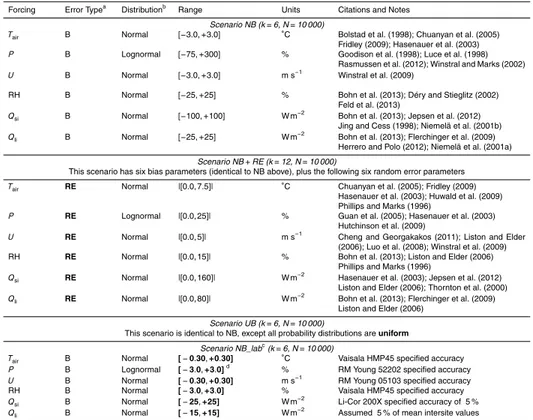
3.2 Forcing error scenarios 15

To test how error characteristics in forcings aﬀ_{ect model outputs, we created four} sce-narios (Fig. 1 and Table 3) with diﬀ_{erent assumptions regarding error types,} distribu-tions, and magnitudes (i.e., error ranges). In the first scenario, only bias (normally or lognormally distributed) was introduced into all forcings at a level of high uncertainty (based on values observed in the field, see Sect. 3.2.3 below). This scenario was

20

named “NB,” where N denotes normal (or lognormal) error distributions and B denotes bias only. The remaining three scenarios were identical to NB except one aspect was changed: scenario NB+_{RE considered both bias and random errors (RE), scenario UB} considered uniformly distributed biases, and scenario NB_lab considered error magni-tudes at minimal values (i.e., specified instrument accuracy as found in a laboratory).

25

(8)

HESSD

11, 13745–13795, 2014

Title Page

Tables Figures

◭ ◮

Back Close

Full Screen / Esc

Discussion

P

a

per

|

Discussion

P

a

per

|

Discussion

P

a

per

|

Discussion

P

a

per

|

3.2.1 Error types

Forcing data inevitably have some (unknown) combination of bias and random errors. However, hydrologic sensitivity analyses have tended to focus more on bias with little or no attention to random errors (Raleigh and Lundquist, 2012), and rarely any consider-ation of interactions between error types. Lapo et al. (2014) tested biases and random

5

errors inQ_siandQ_li forcings, finding that biases generally introduced more variance in modeled SWE than random errors. Their experiment considered biases and random errors separately (i.e., no error interactions allowed), and examined only a subset of the required forcings (i.e., radiation). Here, we examined co-existing biases in all forc-ings in NB, UB, and NB_Lab, and co-existing biases and random errors in all forcforc-ings

10

in NB+_RE.

Table 3 shows the assignment of error types for the four scenarios. We relied on studies that assess errors in measurements or estimated forcings to identify typical characteristics of biases and random errors. Published bias values were more straight-forward to interpret than random errors because common metrics, such as root mean

15

squared error (RMSE) and mean absolute error (MAE), encapsulate both systematic and random errors. Hence, when defining random errors, published RMSE and MAE served as qualitative guidelines.

3.2.2 Error distributions

Error distributions (Table 3) were the same across scenarios NB, NB+_{RE, and NB_lab.}

20

The UB scenario adopted a naive hypothesis that the probability distribution of biases was uniform, a common assumption in sensitivity analyses. However, a uniform dis-tribution implies that extreme and small biases are equally probable. It is likely that error distributions more closely resemble non-uniform distributions (e.g., normal distri-butions) in reality.

25

(9)

HESSD

11, 13745–13795, 2014

Title Page

Tables Figures

◭ ◮

Back Close

Full Screen / Esc

Discussion

P

a

per

|

Discussion

P

a

per

|

Discussion

P

a

per

|

Discussion

P

a

per

|

(Mardikis et al., 2005; Phillips and Marks, 1996), as do Q_si and Q_li errors (T. Bohn, personal communication, 2014). Conflicting reports over the distribution ofU indicated that errors may be approximated with a normal (Phillips and Marks, 1996), a lognormal (Mardikis et al., 2005), or a Weibull distribution (Jiménez et al., 2011). For simplicity, we assumed thatU errors were normally distributed. Finally, we assumedP errors

fol-5

lowed a lognormal distribution to account for snow redistribution due to wind drift/scour (Liston, 2004). Error distributions were truncated in cases when the introduced errors violated physical limits (e.g., negativeU; see Sect. 3.3.5).

3.2.3 Error magnitudes

We considered two magnitudes of forcing uncertainty: levels of uncertainty found in the

10

(1) field vs. (2) a controlled laboratory setting (Table 3). Field and laboratory cases were considered because they sampled realistic errors and minimum errors, respectively. We expected that the error ranges exerted a major control on model uncertainty and sensitivity.

NB, NB+_{RE, and UB considered field uncertainties. Field uncertainties depend on}

15

the source of forcing data and on local conditions (e.g., Flerchinger et al., 2009). To generalize the analysis, we chose error ranges that enveloped the reported uncertainty of diﬀ_{erent methods for acquiring forcing data.}_T_air _{error ranges spanned errors in} mea-surements (Huwald et al., 2009) and commonly used models, such as lapse rates and statistical methods, (Bolstad et al., 1998; Chuanyan et al., 2005; Fridley, 2009;

Hase-20

nauer et al., 2003; Phillips and Marks, 1996).P error ranges spanned undercatch (e.g., Rasmussen et al., 2012) and drift/scour errors. Because UEB lacks dynamic wind re-distribution, accumulation uncertainty was not linked toU but instead toP errors (e.g., drift factor, Luce et al., 1998). Results were thus most relevant to areas with prominent snow redistribution (e.g., alpine zone).U error ranges spanned errors in topographic

25

(10)

HESSD

11, 13745–13795, 2014

Title Page

Tables Figures

◭ ◮

Back Close

Full Screen / Esc

Discussion

P

a

per

|

Discussion

P

a

per

|

Discussion

P

a

per

|

Discussion

P

a

per

|

2013; Feld et al., 2013).Q_si error ranges spanned errors in empirical methods (Bohn et al., 2013), radiative transfer models (Jing and Cess, 1998), satellite-derived prod-ucts (Jepsen et al., 2012), and NWP models (Niemelä et al., 2001b).Q_li error ranges spanned errors in empirical methods (Bohn et al., 2013; Flerchinger et al., 2009; Her-rero and Polo, 2012) and NWP models (Niemelä et al., 2001a).

5

In contrast, scenario NB_lab assumed laboratory levels of uncertainty for each forc-ing. These uncertainty levels vary with the type and quality of sensors, as well as re-lated accessories (e.g., wind shield for aP gauge), which we did not explicitly consider. We assumed that the manufacturers’ specified accuracy of meteorological sensors at a typical SNOw TELemetry (SNOTEL) (Serreze et al., 1999) site in the western USA

10

were representative of minimum uncertainties in forcings because of the widespread use of SNOTEL data in snow studies. While we used the specified accuracy for P

measurements in NB_lab, we note that the instrument uncertainty of±3 % was likely unrepresentative of errors likely to be encountered. For example, corrections applied to theP data (see Sect. 2) exceeded this uncertainty by factors of 3 to 20.

15

3.3 Sensitivity analysis

Numerous approaches that explore uncertainty in numerical models have been de-veloped in the literature of statistics (Christopher Frey and Patil, 2002), environmental modeling (Matott et al., 2009), and hydrology model optimization/calibration (Beven and Binley, 1992; Duan et al., 1992; Kavetski et al., 2002, 2006a, b; Kuczera et al.,

20

2010; Vrugt et al., 2008a, b). Among these, global sensitivity analysis is an elegant platform for testing the impact of input uncertainty on model outputs and for ranking the relative importance of inputs while considering co-existing sources of uncertainty. Global methods are ideal for non-linear models (e.g., snow models). The Sobol (1990) (hereafter Sobol’) method is a robust global method based on the decomposition of

25

(11)

HESSD

11, 13745–13795, 2014

Title Page

Tables Figures

◭ ◮

Back Close

Full Screen / Esc

Discussion

P

a

per

|

Discussion

P

a

per

|

Discussion

P

a

per

|

Discussion

P

a

per

|

3.3.1 Overview

One can visualize any hydrology or snow model as:

Y=_M₍_F_,_θ₎ ₍₁₎

whereYis a matrix of model outputs (e.g., SWE),M( ) is the model operator,Fis a ma-trix of forcings (e.g.,T_air,P,U, etc.), andθis an array of model parameters (e.g., snow

5

surface roughness). The goal of sensitivity analysis is to quantify how variance (i.e., uncertainty) in specific input factors (F and θ) influences variance in specific outputs (Y). Sensitivity analyses tend to focus more on the model parameter array (θ) than on the forcing matrix (Foglia et al., 2009; Herman et al., 2013; Li et al., 2013; Nossent et al., 2011; Rakovec et al., 2014; Rosero et al., 2010; Rosolem et al., 2012; Tang et al.,

10

2007; van Werkhoven et al., 2008). Here, we extend the sensitivity analysis framework to forcing uncertainty by creatingk new parameters (θ₁,θ₂,. . .θ_k) that specify forcing uncertainty characteristics (Vrugt et al., 2008b). By fixing the original model parameters (Table 2), we focus solely on the influence of forcing errors on model output (Y). Note it is possible to consider uncertainty in both forcings and parameters in this framework.

15

3.3.2 Sobol’ sensitivity analysis

Sobol’ sensitivity analysis uses variance decomposition to attribute output variance to input variance. First-order and higher-order sensitivities can be resolved; here, only the total-order sensitivity is examined (see below). The Sobol’ method is advantageous in that it is model independent, can handle non-linear systems, and is among the most

20

robust sensitivity methods (Saltelli and Annoni, 2010; Saltelli, 1999). The primary limi-tation of Sobol is that it is compulimi-tationally intensive, requiring a large number of sam-ples to account for variance across the full parameter space. Below, we describe the methodology but note Saltelli and Annoni (2010) provide an excellent overview for de-signing a Sobol’ sensitivity analysis.

(12)

HESSD

11, 13745–13795, 2014

Title Page

Tables Figures

◭ ◮

Back Close

Full Screen / Esc

Discussion

P

a

per

|

Discussion

P

a

per

|

Discussion

P

a

per

|

Discussion

P

a

per

|

3.3.3 Sensitivity indices and sampling

Within the Sobol’ global sensitivity analysis framework, the total-order sensitivity in-dex (S_T_i) describes the variance in model outputs (Y) due to a specific parameter (θ_i), including both unique (i.e., first-order) eﬀ_{ects and all interactions with all other} param-eters:

5

S_T_i =E[V(Y|θ∼i)]

V(Y) =1−

V[E(Y|θ_∼_i)]

V(Y) (2)

whereE is the expectation (i.e., average) operator,V is the variance operator, andθ_∼_i

signifies all parameters exceptθ_i. The latter expression defines S_T_i as the variance remaining in Y after accounting for variance due to all other parameters (θ_∼_i). S_T_i

values have a range of [0, 1]. Interpretation ofS_T_i values was straightforward because

10

they explicitly quantified the variance introduced to model output by each parameter (i.e., forcing errors). As an example, anS_T_i value of 0.7 for bias parameterθ_i on output

Y_j indicates 70 % of the output variance was due bias in forcing i (including unique eﬀ_{ects and interactions).}

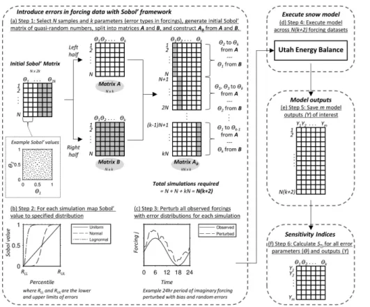
Selecting points in the k-dimensional space for calculating S_T_i was achieved

us-15

ing the quasi-random Sobol’ sequence (Saltelli and Annoni, 2010). The sequence has a uniform distribution in the range [0, 1]. Figure 2a shows an example Sobol’ sequence in two dimensions.

Evaluation of Eq. (2) requires two sampling matrices, which we built with the Sobol’ sequence and refer to as matrices Aand B (Fig. 2a). To construct Aand B, we first

20

specified the number of samples (N) in the parameter space and the number of pa-rameters (k), depending on the error scenario (Table 3). For each scenario and site, we generated a (N×2k) Sobol’ sequence matrix with quasi-random numbers in the [0, 1] range, and then divided it in two parts such that matricesAandBwere each distinct (N xk) matrices. Calculation of S_T_i required perturbing parameters; therefore, a third

25

(13)

HESSD

11, 13745–13795, 2014

Title Page

Tables Figures

◭ ◮

Back Close

Full Screen / Esc

Discussion

P

a

per

|

Discussion

P

a

per

|

Discussion

P

a

per

|

Discussion

P

a

per

|

A, except the ith column, which was from theith column of B, resulting in a (kN x k) matrix (Fig. 2a). Section 3.3.5 provides specific examples of this implementation.

A number of numerical methods are available for evaluating sensitivity indices (Saltelli and Annoni, 2010). From Eq. (2), we computeS_T_i as (Jansen, 1999; Saltelli and Annoni, 2010):

5

S_T_i =

1 2N

PN

j=1

f(A)j−f

AB

(i)

j

2

V(Y) (3)

wheref(A) is the model output evaluated on theAmatrix,f(AB

(i)

) is the model output evaluated on theABmatrix where theith column is from theBmatrix, andi designates

the parameter of interest. Evaluation ofS_T_i required N(k+_{2) simulations at each site} and scenario.

10

3.3.4 Bootstrapping of sensitivity indices

To test the reliability ofS_T_i, we used bootstrapping with replacement across theN(k+ 2) outputs, similar to Nossent et al. (2011). The mean and 95 % confidence interval were calculated using the Archer et al. (1997) percentile method and 10 000 samples. For all cases, finalS_T_i values were generally close to the mean bootstrapped values,

15

suggesting convergence. Thus, we report only the mean and 95 % confidence intervals of the bootstrappedS_T_i values.

3.3.5 Workflow and error introduction

Figure 2 shows the workflow for creating the Sobol’A,B, andABmatrices, converting

Sobol’ values to errors, applying errors to the original forcing data, executing the model

20

(14)

HESSD

11, 13745–13795, 2014

Title Page

Tables Figures

◭ ◮

Back Close

Full Screen / Esc

Discussion

P

a

per

|

Discussion

P

a

per

|

Discussion

P

a

per

|

Discussion

P

a

per

|

Step 1) Generate an initial (N×2k) Sobol’ matrix (with N and k values for each scenario, Table 3), separate into A and B, and construct AB (Fig. 2a). NB+RE had k=_{12 (six bias and six random error parameters). All other scenarios had} _k=_{6 (all} bias parameters).

Step 2) In each simulation, map the Sobol’ value of each forcing error parameter

5

(θ) to the specified error distribution and range (Fig. 2b, Table 3). For example, θ= 0.75 would map to a Q_si bias of +_{50 W m}−2 _{for a uniform distribution in the range} [−100 W m−2,+_{100 W m}−2_].

Step 3) In each simulation, perturb (i.e., introduce artificial errors) the observed time series of theith forcing (F_i) with bias (all scenarios), or both bias and random errors

10

(NB+_{RE only) (Fig. 2c):}

F_i′=_F

iθB,ibi+(Fi+θB,i)(1−bi)+θRE,iRci (4)

whereF_i′is the perturbed forcing time series,θ_B,_i is the bias parameter for forcingi,b_i

is a binary switch indicating multiplicative bias (b_i =_{1) or additive bias (}_b_i =_0), _θ_RE,_i is the random error parameter for forcingi,R is a time series of randomly distributed

15

noise (normal distribution, mean=_{0) scaled in the [−1, 1] range, and} _c_i _{is a binary} switch indicating whether random errors are introduced (c_i=_{1 in scenario NB}+_RE andc_i =_{0 in all other scenarios). For}_T

air,U, RH,Qsi, andQli,bi =0; forP,bi =1. For

P,U, andQ_si, we restricted random errors to periods with positive values. We checked

F_i′for non-physical values (e.g., negativeQ_si) and set these to physical limits. This was

20

most common when perturbing U, RH, andQ_si; negative values of perturbedP only occurred when random errors were considered (Eq. 4). Due to this resetting of non-physical errors, the error distribution was truncated (i.e., it was not always possible to impose extreme errors). Additional tests (not shown) suggested that distribution trun-cation changed sensitivity indices minimally (i.e.,<5 %) and did not alter the relative

25

ranking of forcing errors.

(15)

HESSD

11, 13745–13795, 2014

Title Page

Tables Figures

◭ ◮

Back Close

Full Screen / Esc

Discussion

P

a

per

|

Discussion

P

a

per

|

Discussion

P

a

per

|

Discussion

P

a

per

|

80 000 simulations, for a total of 1 520 000 simulations in the analysis. The doubling ofk in NB+_{RE did not result in twice as many simulations because the number of} simulations scaled asN(k+_2).

Step 5) Save the model outputs for each simulation (Fig. 2e).

Step 6) Calculate S_T_i for each forcing error parameter and model output (Fig. 2f)

5

based on Sects. 3.3.3–3.3.4. Prior to calculatingS_T_i, we screened the model outputs for cases where UEB simulated too little or too much snow (which can occur with per-turbed forcings). For a valid simulation, we required a minimum peak SWE of 50 mm, a minimum continuous snow duration of 15 d, and identifiable snow disappearance. We rejected samples that did not meet these criteria to avoid meaningless or undefined

10

metrics (e.g., peak SWE in ephemeral snow or snow disappearance for a simulation that did not melt out). The number of rejected samples varied with site and scenario (Table 4). On average, 92 % passed the requirements. All cases had at least 86 % satisfactory samples, except in UB at SASP, where only 34 % met the requirements. Despite this attrition,S_T_i values still converged in all cases.

15

4 Results

4.1 Uncertainty propagation to model outputs

Figure 3 shows density plots of daily SWE from UEB at the four sites and four forcing error scenarios (Fig. 1, Table 3), while Fig. 4 summarizes the model outputs. As a re-minder, NB assumed normal (or lognormal) biases at field level uncertainty. The other

20

scenarios were the same as NB, except NB+_{RE considered both biases and random} errors, UB considered uniform distributions, and NB_lab considered lower error mag-nitudes (i.e., laboratory level uncertainty).

Large uncertainties in SWE were evident, particularly in NB, NB+_{RE, and UB} (Fig. 3a–l). The large range in modeled SWE within these three scenarios often

trans-25

(16)

HESSD

11, 13745–13795, 2014

Title Page

Tables Figures

◭ ◮

Back Close

Full Screen / Esc

Discussion

P

a

per

|

Discussion

P

a

per

|

Discussion

P

a

per

|

Discussion

P

a

per

|

(Fig. 4i–l) and total sublimation (Fig. 4m–p). In contrast, SWE and output uncertainty in NB_lab was comparatively small (Figs. 3m–p and 4). The envelope of SWE simula-tions in NB_lab generally encompassed observed SWE at all sites, except during early winter at IC (Fig. 3m), which was possibly due to initialP data quality and redistribu-tion of snow to the snow pillow site. NB_lab simularedistribu-tions were expected to encompass

5

observed SWE due to the adjustments made to the originalP data (see Sect. 2). NB and NB+_{RE generally yielded similar SWE density plots (Fig. 3a–h), but} NB+_{RE yielded a higher frequency of extreme SWE simulations. NB and NB}+_RE also had very similar (but not equivalent) mean outputs values and ensemble spreads at all sites except IC (Fig. 4). This initial observation suggested that forcing biases

con-10

tributed more to model uncertainty than random errors at CDP, RME, and SASP. IC may have had higher sensitivity to random errors due to the low snow accumulation at that site and brief snowmelt season (less than 10 d).

NB and UB yielded generally very diﬀ_{erent model outputs (Figs. 3 and 4). The only} diﬀ_{erence in these two scenarios was the assumption regarding error distribution}

(Ta-15

ble 3). Uniformly distributed forcing biases (scenario UB) yielded a more uniform en-semble of SWE simulations (Fig. 3i–l), larger mean values of peak SWE and ablation rates, and later snow disappearance, as well as larger uncertainty ranges in all out-puts. At some sites, UB also had a higher frequency of simulations where seasonal sublimation was negative.

20

Relative to NB, NB_lab had smaller uncertainty ranges in all model outputs (Figs. 3 and 4), an expected result given the lower magnitudes in forcing errors in NB_lab (Ta-ble 3). Likewise, NB_lab SWE simulations were generally less biased than NB, relative to observations (Fig. 3). NB_lab generally had higher mean peak SWE and ablation rates, and later mean snow disappearance timing than NB (Fig. 4).

(17)

HESSD

11, 13745–13795, 2014

Title Page

Tables Figures

◭ ◮

Back Close

Full Screen / Esc

Discussion

P

a

per

|

Discussion

P

a

per

|

Discussion

P

a

per

|

Discussion

P

a

per

|

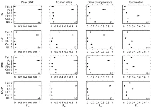
4.2 Model sensitivity to forcing error characteristics

Total-order (S_T_i) sensitivity indices from the Sobol’ sensitivity analysis are shown in Figs. 5–8 for the four scenarios. In these figures, “B” signifies bias and “RE” signifies random errors. Results from each scenario are described below.

Scenario NB showed that UEB peak SWE was most sensitive toP bias at all sites,

5

with S_T_i values ranging from 0.90 to 1.00 (Fig. 5a–d). P bias was also the most im-portant factor for ablation rates and snow disappearance at all sites in scenario NB (Fig. 5e–l). After P bias, T_air bias was the next most important factor at CDP while biases inQ_si andQ_li were secondarily important at RME (Fig. 5f and g). In NB, subli-mation was most sensitive to RH bias at IC, CDP, and RME, while at SASP sublisubli-mation

10

was most sensitive toUbias (Fig. 5m–p).Q_siandQ_libiases were secondarily important to sublimation at IC and CDP, whileT_air bias had secondary importance at RME and SASP.

At all sites in NB+_{RE, peak SWE was most sensitive to}_P _{bias, with}_S_T_i _{ranging from} 0.95 to 1.00 (Fig. 6a–d). At CDP, RME, and SASP in NB+_{RE, ablation rates and snow}

15

disappearance were also most sensitive toP bias, withS_T_i ranging from 0.94 to 1.00 (ablation rates) and 0.74 to 0.93 (snow disappearance). At IC, no single error emerged as a dominant control on ablation rates, while snow disappearance was most sensitive toQ_li bias (S_T_i =_{0.75). Sublimation in NB}+_{RE was most sensitive to di}ﬀ_{erent errors at} each site, where the dominant factors were RH bias at IC,Q_li bias at CDP,T_air bias at

20

RME, andU bias at SASP (Fig. 6m–p).

At all sites in UB, P bias was most important for peak SWE, ablation rates, and snow disappearance (Fig. 7a–l). The only exception was at IC, where ablation rates had similar sensitivity toP bias andU bias. Sublimation was most sensitive to RH bias at IC, CDP, and RME, andU bias as SASP (Fig. 7m–p). For sublimation in UB,Q_libias

25

(18)

HESSD

11, 13745–13795, 2014

Title Page

Tables Figures

◭ ◮

Back Close

Full Screen / Esc

Discussion

P

a

per

|

Discussion

P

a

per

|

Discussion

P

a

per

|

Discussion

P

a

per

|

Relative to the other scenarios, NB_lab portrayed diﬀ_{erent model sensitivities to} forc-ing errors (Fig. 8). Across all sites and outputs,Q_li bias was consistently the most im-portant factor. This was surprising, given that the bias magnitudes were lower forQ_li

than for Q_si (Table 3). Whereas P bias was often important for peak SWE, ablation rates, and snow disappearance in the other scenarios,P bias was seldom important

5

in NB_lab (main exception was peak SWE at IC, Fig. 8a). This was due to the discrep-ancy between the specified accuracy forP gauges and typical errors encountered in the field (Rasmussen et al., 2012; Sieck et al., 2007).

4.3 Impact of error types

Figure 9 compares the mean S_T_i values (above) from NB and NB+_{RE to test how}

10

forcing error type aﬀ_{ects model sensitivity. In this test, only the six bias parameters} from NB+_{RE were compared, as these were found in both scenarios. Across sites and} model outputs,S_T_i values were higher in NB+_{RE than NB. This suggested that random} errors interact with bias, thereby increasing model sensitivity to bias. However, while theS_T_i values diﬀ_{ered between these two scenarios, the overall importance ranking of}

15

forcing biases was generally not altered, and NB oﬀ_{ered the same general conclusions} regarding the relative impacts of biases in the forcings.

4.4 Impact of error distributions

Figure 10 compares mean S_T_i values from NB and UB to test how the distribution of bias influences model outputs.S_T_i values from the two scenarios generally plotted

20

close to the 1:1 line, suggesting good correspondence in the sensitivity of UEB under diﬀ_{erent bias distributions. In other words, the error distribution had little impact on} model sensitivity to forcing errors. With a few exceptions where sensitivities of less important terms were clustered (e.g., Fig. 10e), the hierarchy of forcing biases was similar between these two scenarios.

(19)

HESSD

11, 13745–13795, 2014

Title Page

Tables Figures

◭ ◮

Back Close

Full Screen / Esc

Discussion

P

a

per

|

Discussion

P

a

per

|

Discussion

P

a

per

|

Discussion

P

a

per

|

4.5 Impact of error magnitude

Figure 11 compares mean S_T_i values from NB and NB_lab to test the importance of forcing error magnitudes to model output. The results showed that the total sensitiv-ity of model outputs to forcing biases depended substantially on the levels of forcing uncertainty considered. As a primary example, the scenarios did not agree whetherP 5

bias orQ_li bias was the most important factor for peak SWE, ablation rates, and snow disappearance dates at all four sites (Fig. 11a–l). At IC and SASP, peak SWE sensi-tivity to the secondary forcings (i.e., forcings most important after the most important factor) was greater in NB_lab than NB. In contrast, sublimation was more sensitive to the secondary forcings in NB than NB_lab.

10

5 Discussion

Here we have examined the sensitivity of physically based snow simulations to forcing error characteristics (i.e., types, distributions, and magnitudes) using Sobol’ global sen-sitivity analysis. Among these characteristics, the magnitude of biases had the most significant impact on UEB simulations (Figs. 3–4) and on model sensitivity (Fig. 11).

15

Random errors were important in that they introduced more interactions in the uncer-tainty space, as evident in the higherS_T_i values in scenario NB+_{RE vs. NB (Fig. 9),} but they were rarely among the most important factors for the model outputs at the sites (Fig. 6). The assumed distribution of biases was important in that it increased the range of model outputs (compare NB and UB in Fig. 4), but this did not often translate

20

to diﬀ_{erent model sensitivity to forcing errors (Fig. 10).}

Our central argument at the onset was that forcing uncertainty may be comparable to parametric and structural uncertainty in snow-aﬀ_{ected catchments. To support our} argument, we compare our results at CDP in 2005–2006 to Essery et al. (2013), who assessed the impact of structural uncertainty on SWE simulations from 1701 physically

25

(20)

HESSD

11, 13745–13795, 2014

Title Page

Tables Figures

◭ ◮

Back Close

Full Screen / Esc

Discussion

P

a

per

|

Discussion

P

a

per

|

Discussion

P

a

per

|

Discussion

P

a

per

|

j, n) to the corresponding ensemble in Fig. 10 of Essery et al. (2013), it is clear that the forcing uncertainty considered in most scenarios here overwhelms the structural uncertainty at this site. Whereas the 1701 models in Essery et al. (2013) generally have peak SWE between 325–450 mm, the 95 % interval due to forcing uncertainty spans 100–565 mm in NB, 110–580 mm in NB+_{RE, 125–1880 mm in UB, and 370–430 mm}

5

in NB_lab (Fig. 4b). Spread in snow disappearance due to structural uncertainty spans mid-April to early-May in Essery et al. (2013), but the range of snow disappearance due to forcing uncertainty spans late-March to early-May in NB and NB+_RE, late-March to early July in UB, and mid-April to early-May in NB_lab (Fig. 4j). Structural uncertainty is less impactful on model outputs at this site than the forcing uncertainty

10

of NB, NB+_{RE, and UB, and is only marginally more impactful than the minimal forcing} uncertainty tested in NB_lab. Thus, forcing uncertainty cannot always be discounted, and the magnitude of forcing uncertainty is a critical factor in how forcing uncertainty compares to parametric and structural uncertainty.

It could be argued that forcing uncertainty only appears greater than structural

un-15

certainty in the CDP example because of the largeP error magnitudes (Table 3), which are representative of barren areas with drifting snow (e.g., alpine areas, cold prairies) but perhaps not representative of sheltered areas (e.g., forest clearings). To check this, we conducted a separate test (no figures shown) replicating scenario NB with smaller

P biases ranging from−10 to+_{10 %. This}_P _{uncertainty range was selected because}

20

Meyer et al. (2012) found 95 % of SNOTEL sites (often in forest clearings) had ob-servations of accumulated P within 20 % of peak SWE. This test resulted in a 95 % peak SWE interval of 228–426 mm and a 95 % snow disappearance interval spanning early-April to early-May. These ranges were still larger than the ranges due to struc-tural uncertainty (Essery et al., 2013), further demonstrating the importance of forcing

25

uncertainty in snow-aﬀ_{ected areas.}

(21)

(Du-HESSD

11, 13745–13795, 2014

Title Page

Tables Figures

◭ ◮

Back Close

Full Screen / Esc

Discussion

P

a

per

|

Discussion

P

a

per

|

Discussion

P

a

per

|

Discussion

P

a

per

|

rand and Margulis, 2008; He et al., 2011a; Schmucki et al., 2014). However, we note wind uncertainty in snow-aﬀ_{ected areas can also be important to snowpack dynamics} through drift/scour processes (Mott and Lehning, 2010; Winstral et al., 2013), and our “drift factor” formulation (Luce et al., 1998) did not account for the role of wind inP un-certainty. Thus,U is likely more important than the results suggest. Future work could

5

account for this by assigningP errors that are correlated withU.

It was surprising thatP bias was often the most critical forcing error for ablation rates (Figs. 5–7). This is contrary to other studies that have suggested the most important factors for snowmelt are radiation, wind, humidity, and temperature (e.g., Zuzel and Cox, 1975). Ablation rates were highly sensitive to P bias because it controlled the

10

timing and length of the ablation season. Positive (negative)P bias extends (truncates) the fraction of the ablation season in the warmest summer months when ablation rates and radiative energy approach maximum values. Trujillo and Molotch (2014) reported a similar result based on SNOTEL observations.

While peak SWE, ablation rates, and snow disappearance dates had similar

sensitiv-15

ities to forcing errors (particularly toP biases), sublimation exhibited notably diﬀ_erent sensitivity to forcing errors. P bias was frequently the least important factor for sub-limation, in contrast to the other model outputs. In only a few cases (e.g., all sites in NB+_RE),_P _{errors explained more than 5 % of uncertainty in modeled sublimation, and} these cases were likely tied to the control ofP on snowpack duration (when sublimation

20

is possible). Biases in RH,U, andT_air were often the major controls on modeled sub-limation in the field uncertainty scenarios (i.e., NB, NB+_{RE, and UB), while} _Q_li _bias controlled modeled sublimation in the lab uncertainty scenario (i.e., NB_lab). These results partially agree with the sensitivity analysis of Lapp et al. (2005), who showed the most important forcings for sublimation in the Canadian Rockies wereU and Q_si.

25

These results suggest that no single forcing is important across all modeled variables, and model sensitivity strongly depends on the output of interest.

(22)

un-HESSD

11, 13745–13795, 2014

Title Page

Tables Figures

◭ ◮

Back Close

Full Screen / Esc

Discussion

P

a

per

|

Discussion

P

a

per

|

Discussion

P

a

per

|

Discussion

P

a

per

|

certainties in forcing data. The results also identify the need for continued research in constrainingP uncertainty in snow-aﬀ_{ected catchments. This may be achieved using} advanced pathways for quantifying snowfall precipitation, such as NWP models (Ras-mussen et al., 2011, 2014). However, in a broader sense, the hydrologic community should consider whether deterministic forcings (i.e., single time series for each forcing)

5

are a reasonable practice for physically based models, given the large uncertainties in both future (e.g., climate change) and historical data (especially in poorly moni-tored catchments) and the complexities of hydrologic systems (Gupta et al., 2008). We suggest that probabilistic model forcings (e.g., Clark and Slater, 2006) present one po-tential path forward where measures of forcing uncertainty can be explicitly included in

10

the forcing datasets. The challenges are (1) to ensure statistical reliability in our under-standing of forcing errors and (2) to assess how best to input probabilistic forcings into current model architectures.

Limitations of the analysis are (1) we do not consider parametric and structural un-certainty and (2) we only consider a single model and sensitivity analysis method. We

15

expect diff_{erent snow models may yield di}ff_{erent sensitivities to forcing uncertainty. For} example, both Koivusalo and Heikinheimo (1999) and Lapo et al. (2014) found UEB (Tarboton and Luce, 1996) and the SNTHERM model (Jordan, 1991) exhibited signifi-cant diff_{erences in radiative and turbulent heat exchange. In other models, we expect}_P biases would still dominate peak SWE, ablation rates, and snow disappearance timing,

20

but we might expect diff_{erent sensitivities to other forcing errors. Likewise, it is possible} that diff_{erent sensitivity analysis methods might yield di}ff_{erent results than the Sobol’} method (Pappenberger et al., 2008).

Finally, while the Sobol’ method is often considered the “baseline” method in global sensitivity analysis, we note that it comes at a relatively high computation cost

25

(23)

HESSD

11, 13745–13795, 2014

Title Page

Tables Figures

◭ ◮

Back Close

Full Screen / Esc

Discussion

P

a

per

|

Discussion

P

a

per

|

Discussion

P

a

per

|

Discussion

P

a

per

|

sensitivity analyses that concurrently consider uncertainty in forcings, parameters, and structure in a hydrologic model will be more feasible in the future with better computing resources and advances in sensitivity analysis methods.

6 Conclusions

Application of the Sobol’ sensitivity analysis framework across sites in contrasting snow

5

climates reveals that forcing uncertainty can significantly impact model behavior in snow-aﬀ_{ected catchments. Model output uncertainty due to forcings can be} compa-rable to or larger than model uncertainty due to model structure. Key considerations in model sensitivity to forcing errors are the magnitudes of forcing errors and the outputs of interest. For the sensitivity of the model tested, random errors in forcings are

gener-10

ally less important than biases, and the distribution of biases is relatively less important than the magnitude of biases.

The analysis shows how forcing uncertainty might be included in a formal sensitivity analysis framework through the introduction of new parameters that specify the char-acteristics of forcing uncertainty. The framework could be extended to other physically

15

based models and sensitivity analysis methodologies, and could be used to quantify how uncertainties in model forcings and parameters interact. In future work, it would be interesting to assess the interplay between co-existing uncertainties in forcing errors, model parameters, and model structure, and to test how model sensitivity changes relative to all three sources of uncertainty.

20

Author contributions. The National Center for Atmospheric Research is sponsored by the

Na-tional Science Foundation.

Acknowledgements. M. Raleigh was supported by a post-doctoral fellowship in the Advanced

Study Program at the National Center for Atmospheric Research (sponsored by NSF). J. Lundquist was supported by NSF (EAR-838166 and EAR-1215771). Thanks to M. Sturm, G. 25

(24)

HESSD

11, 13745–13795, 2014

Title Page

Tables Figures

◭ ◮

Back Close

Full Screen / Esc

Discussion

P

a

per

|

Discussion

P

a

per

|

Discussion

P

a

per

|

Discussion

P

a

per

|

Landry for assistance with Swamp Angel data, and E. Gutmann and P. Mendoza for feedback. For Imnavait Creek data, we acknowledge US Army Cold Regions Research and Engineering Laboratory, the NSF Arctic Observatory Network (AON) Carbon, Water, and Energy Flux mon-itoring project and the Marine Biological Laboratory, Woods Hole, and the University of Alaska, Fairbanks. The experiment was improved thanks to conversations with D. Slater.

5

References

Archer, G. E. B., Saltelli, A., and Sobol, I. M.: Sensitivity measures,anova-like techniques and the use of bootstrap, J. Stat. Comput. Sim., 58, 99–120, doi:10.1080/00949659708811825, 1997. 13757

Bales, R. C., Molotch, N. P., Painter, T. H., Dettinger, M. D., Rice, R., and Dozier, J.: 10

Mountain hydrology of the western United States, Water Resour. Res., 42, W08432, doi:10.1029/2005WR004387, 2006. 13747

Barnett, T. P., Pierce, D. W., Hidalgo, H. G., Bonfils, C., Santer, B. D., Das, T., Bala, G., Wood, A. W., Nozawa, T., Mirin, A. A., Cayan, D. R., and Dettinger, M. D.: Human-induced changes in the hydrology of the western United States, Science, 319, 1080–1083, 15

doi:10.1126/science.1152538, 2008. 13746

Bastola, S., Murphy, C., and Sweeney, J.: The role of hydrological modelling uncertainties in climate change impact assessments of Irish river catchments, Adv. Water Resour., 34, 562– 576, doi:10.1016/j.advwatres.2011.01.008, 2011. 13747

Benke, K. K., Lowell, K. E., and Hamilton, A. J.: Parameter uncertainty, sensitivity analysis and 20

prediction error in a water-balance hydrological model, Math. Comput. Model., 47, 1134– 1149, doi:10.1016/j.mcm.2007.05.017, 2008. 13747

Beven, K. and Binley, A.: The future of distributed models: model calibration and uncertainty prediction, Hydrol. Process., 6, 279–298, doi:10.1002/hyp.3360060305, 1992. 13747, 13754 Bohn, T. J., Livneh, B., Oyler, J. W., Running, S. W., Nijssen, B., and Lettenmaier, D. P.: Global 25

(25)

HESSD

11, 13745–13795, 2014

Title Page

Tables Figures

◭ ◮

Back Close

Full Screen / Esc

Discussion

P

a

per

|

Discussion

P

a

per

|

Discussion

P

a

per

|

Discussion

P

a

per

|

Bolstad, P. V., Swift, L., Collins, F., and Régnière, J.: Measured and predicted air temperatures at basin to regional scales in the southern Appalachian mountains, Agr. Forest Meteorol., 91, 161–176, doi:10.1016/S0168-1923(98)00076-8, 1998. 13753, 13783

Bret-Harte, S., Shaver, G., and Euskirchen, E.: Eddy Flux Measurements, Ridge Sta-tion, Imnavait Creek, Alaska – 2010, Long Term Ecological Research Network, 5

doi:10.6073/pasta/fb047eaa2c78d4a3254bba8369e6cee5, 2010a. 13749

Bret-Harte, S., Shaver, G., and Euskirchen, E.: Eddy Flux Measurements, Fen Sta-tion, Imnavait Creek, Alaska – 2010, Long Term Ecological Research Network, doi:10.6073/pasta/dde37e89dab096bea795f5b111786c8b, 2010b. 13749

Bret-Harte, S., Euskirchen, E., Griﬃ_{n, K., and Shaver, G.: Eddy Flux Measurements,} Tus-10

sock Station, Imnavait Creek, Alaska – 2011, Long Term Ecological Research Network, doi:10.6073/pasta/44a62e0c6741b3bd93c0a33e7b677d90, 2011a. 13749

Bret-Harte, S., Euskirchen, E., and Shaver, G.: Eddy Flux Measurements, Fen Sta-tion, Imnavait Creek, Alaska – 2011, Long Term Ecological Research Network, doi:10.6073/pasta/50e9676f29f44a8b6677f05f43268840, 2011b. 13749

15

Bret-Harte, S., Euskirchen, E., and Shaver, G.: Eddy Flux Measurements, Ridge Sta-tion, Imnavait Creek, Alaska – 2011, Long Term Ecological Research Network, doi:10.6073/pasta/5d603c3628f53f494f08f895875765e8, 2011c. 13749

Burles, K. and Boon, S.: Snowmelt energy balance in a burned forest plot, Crowsnest Pass, Alberta, Canada, Hydrol. Process., 25, 3012–3029, doi:10.1002/hyp.8067, 2011. 13748 20

Butts, M. B., Payne, J. T., Kristensen, M., and Madsen, H.: An evaluation of the impact of model structure on hydrological modelling uncertainty for streamflow simulation, J. Hydrol., 298, 242–266, doi:10.1016/j.jhydrol.2004.03.042, 2004. 13747

Cheng, F.-Y. and Georgakakos, K. P.: Statistical analysis of observed and simulated hourly surface wind in the vicinity of the Panama Canal, Int. J. Climatol., 31, 770–782, 25

doi:10.1002/joc.2123, 2011. 13753, 13783

Christopher Frey, H. and Patil, S. R.: Identification and review of sensitivity analysis methods, Risk Anal., 22, 553–578, doi:10.1111/0272-4332.00039, 2002. 13754

Chuanyan, Z., Zhongren, N., and Guodong, C.: Methods for modelling of temporal and spatial distribution of air temperature at landscape scale in the southern Qilian mountains, China, 30

Ecol. Model., 189, 209–220, doi:10.1016/j.ecolmodel.2005.03.016, 2005. 13753, 13783 Clark, M. P. and Slater, A. G.: Probabilistic quantitative precipitation estimation in complex

(26)

HESSD

11, 13745–13795, 2014

Title Page

Tables Figures

◭ ◮

Back Close

Full Screen / Esc

Discussion

P

a

per

|

Discussion

P

a

per

|

Discussion

P

a

per

|

Discussion

P

a

per

|

Clark, M. P., Slater, A. G., Rupp, D. E., Woods, R. A., Vrugt, J. A., Gupta, H. V., Wagener, T., and Hay, L. E.: Framework for Understanding Structural Errors (FUSE): a modular framework to diagnose diﬀ_{erences between hydrological models, Water Resour. Res., 44, W00B02,} doi:10.1029/2007WR006735, 2008. 13747

Clark, M. P., Kavetski, D., and Fenicia, F.: Pursuing the method of multiple working hypothe-5

ses for hydrological modeling, Water Resour. Res., 47, 1–16, doi:10.1029/2010WR009827, 2011. 13747

Dadic, R., Mott, R., Lehning, M., Carenzo, M., Anderson, B., and Mackintosh, A.: Sensitivity of turbulent fluxes to wind speed over snow surfaces in diﬀ_{erent climatic settings, Adv. Water} Resour., 55, 178–189, doi:10.1016/j.advwatres.2012.06.010, 2013. 13748

10

Deems, J. S., Painter, T. H., Barsugli, J. J., Belnap, J., and Udall, B.: Combined impacts of cur-rent and future dust deposition and regional warming on Colorado River Basin snow dynam-ics and hydrology, Hydrol. Earth Syst. Sci., 17, 4401–4413, doi:10.5194/hess-17-4401-2013, 2013. 13746

Déry, S. and Stieglitz, M.: A note on surface humidity measurements in the cold Canadian 15

environment, Bound.-Lay. Meteorol., 102, 491–497, doi:10.1023/A:1013890729982, 2002. 13753, 13783

Di Baldassarre, G. and Montanari, A.: Uncertainty in river discharge observations: a quantitative analysis, Hydrol. Earth Syst. Sci., 13, 913–921, doi:10.5194/hess-13-913-2009, 2009. 13747 Duan, Q., Sorooshian, S., and Gupta, V.: Eﬀ_{ective and e}ﬃ_{cient global optimization for} concep-20

tual rainfall-runoﬀ _{models, Water Resour. Res., 28, 1015–1031, doi:10.1029/91WR02985,} 1992. 13754

Durand, M. and Margulis, S. A.: Eﬀ_{ects of uncertainty magnitude and accuracy on assimilation} of multiscale measurements for snowpack characterization, J. Geophys. Res., 113, D02105, doi:10.1029/2007JD008662, 2008. 13748, 13764

25

Elsner, M. M., Gangopadhyay, S., Pruitt, T., Brekke, L. D., Mizukami, N., and Clark, M. P.: How does the choice of distributed meteorological data aﬀ_{ect hydrologic model calibration and} streamflow simulations?, J. Hydrometeorol., 15, 1384–1403, doi:10.1175/JHM-D-13-083.1, 2014. 13747

Essery, R., Morin, S., Lejeune, Y., and B Ménard, C.: A comparison of 1701 snow 30