Development of an acoustic computational software to analyse composite and sandwich panels

(1)

Development of an acoustic computational software to

analyse composite and sandwich panels

Carlos António de Francisco Machado

Thesis submitted to

Faculdade de Engenharia da Universidade do Porto

as a requirement to obtain the MSc degree in Mechanical Engineering.

Under supervision of

Professor Jorge Américo Oliveira Pinto Belinha Professor Aurélio Lima Araújo

Professor Renato Manuel Natal Jorge Professor Lúcia Maria de Jesus Simas Dinis

(2)

(3)

(4)

(5)

Agradecimentos

Ao professor Jorge Belinha, um grande obrigado, não só por todo o apoio, tempo, orientação e ajuda prestadas durante todo o semestre, mas também por me ter dado a oportunidade de realizar esta tese.

Ao professor Renato Natal Jorge, professor Aurélio Araújo e à professora Lúcia Dinis, agradeço pelo esclarecimento de dúvidas assim como a sua disponibilidade em auxiliar em qualquer altura do trabalho. Agradeço também a todos os professores que tive a oportunidade de travar conhecimento e pelos preceitos transmitidos ao longo dos anos que estudei na FEUP.

Obrigado a todos os meus amigos que me acompanharam durante este percurso e que influenciaram de forma positiva a minha formação pessoal e académica. Um obrigado especial aos que estiveram lá nos momentos mais secantes durante as épocas de exames, e que graças a eles todos esses momentos agora dão saudades.

Em especial, gostava de agradecer à minha família, não só por todo o apoio, carinho e alegria que me deram durante todos estes anos, mas sim por serem a principal razão porque todo este meu percurso foi possível.

(6)

(7)

Funding

The author truly acknowledge the funding provided by Ministério da Educação e Ciência – Fundação para a Ciência e a Tecnologia (Portugal), by project funding UID/EMS/50022/2013 – “Advanced materials for noise reduction: modeling, optimization and experimental validation” (funding provided by the inter-institutional projects from LAETA and INEGI). The author truly acknowledges the work conditions provided by the Applied Mechanics Division (SMAp) of the department of mechanical engineering (DEMec) of FEUP and by the project NORTE-01-0145-FEDER-000022 – SciTech – Science and Technology for Competitive and Sustainable Industries, co-financed by Programa Operacional Regional do Norte (NORTE2020), through Fundo Europeu de Desenvolvimento Regional (FEDER).

(8)

(9)

Development of an acoustic computational software to analyse

composite and sandwich panels.

by

Carlos António de Francisco Machado

Thesis submitted in fulfilment of the degree of Master of Science in

Mechanical Engineering in the Faculdade de Engenharia da Universidade do Porto, under the supervision of:

Professor Jorge Américo Oliveira Pinto Belinha

Professor at Faculdade de Engenharia da Universidade do Porto and

Professor Aurélio Lima Araújo

Associated Professor at Instituto Superior Técnico Professor Renato Manuel Natal Jorge

Associated Professor at Faculdade de Engenharia da Universidade do Porto Professor Lúcia Maria de Jesus Simas Dinis

Associated Professor at Faculdade de Engenharia da Universidade do Porto

Abstract

When numerical techniques are used to study structures subjected to dynamic loads, the Finite Element Method (FEM) is usually the method adopted. However, other accurate and efficient numerical methods, such as meshless methods, have been gaining appeal over the last few years. Meshless methods avoid the need to construct elements to assure nodal connectivity, instead it relies on the overlap of “influence-domains”, allowing more freedom on the placement of the nodes and providing a more smooth stress field. In this work, the dynamic and acoustical analysis of structures is extended to two different meshless methods, the RPIM and NNRPIM. For this, algorithms are created respecting both formulations. In the end, several examples, focusing on laminated and sandwich plates and beams, are analysed to verify the accuracy of both methods, and the results compared with those produced by the FEM and documented in the literature.

(10)

(11)

Development of an acoustic computational software to analyse

composite and sandwich panels.

por

Carlos António de Francisco Machado

Tese apresentada à Faculdade de Engenharia da Universidade do Porto, para obtenção do grau de Mestre em Engenharia Mecânica,

sob a orientação de:

Professor Jorge Américo Oliveira Pinto Belinha

Professor da Faculdade de Engenharia da Universidade do Porto e

Professor Aurélio Lima Araújo

Professor Associado do Instituto Superior Técnico Professor Renato Manuel Natal Jorge

Professor Associado da Faculdade de Engenharia da Universidade do Porto Professora Lúcia Maria de Jesus Simas Dinis

Professor Associado da Faculdade de Engenharia da Universidade do Porto

Sumário

Quando métodos numéricos são aplicados no estudo do comportamento de estruturas sujeitas a solicitações dinámicas, o Método dos Elementos Finitos (MEF) é geralmente o processo aplicado. No entanto, outras técnicas númericas, também precisas e eficientes, como os Métodos Sem Malha, tem vindo a gerar grande interesse junto da comunidade cientifica nos ultimos anos. Métodos Sem Malha distinguem-se por não necessitarem de utilizar elementos para garantir a ligação entre os vários nós, para tal, esta conexão é assegurada pela sobreposição dos vários “dominios de influencia”, conferindo a estes métodos mais liberdade na colocação dos nós e a obtenção de campos de tensão mais suaves, dado as tensões não terem que ser interpoladas entre os elementos. Neste trabalho, a analise dinamica e acustica de estruturas é extendida a dois métodos sem malha, o RPIM e o NNRPIM. Para tal, são criados algoritmos para ambas formulações. No final, são resolvidos vários exemplos, focados também na análise de placas e vigas laminadas e em “sandwich”, para demostrar a performance destes dois métodos, sendo os resultados comparados com aqueles produzidos com o MEF e documentados na literatura.

(12)

(13)

(14)

(15)

List of Figures

Figure 1: Typical FRF (Frequency Response Function) of a vibroacoustic system [3]. ... 2

Figure 2: a) Irregular mesh; b) regular mesh [28]. ... 9

Figure 3: Background integration mesh a) nodal independent; b) nodal depedent (Voronӧi diagram) [28]. ... 9

Figure 4: Interpolation function 𝑢ℎ(𝑥) and the discrete nodal parameters (𝑥𝑖) [28]... 11

Figure 5: Triangle of Pascal [28]. ... 12

Figure 6: a) Initial set of nodes of the structure. b) Normal to straight line that connects the closest node to 𝑛0. c) Closed geometry and neighbor nodes. d) Voronoї cell 𝑉0for node 𝑛0 [28]. ... 14

Figure 7: a) First degree influence-cell b) second degree influence cell [28]. ... 15

Figure 8: a) Irregular mesh generating quadrangular areas b) regular mesh generating triangular areas [28]. ... 15

Figure 9: Example of a structure under: a) plane stress; b) plane strain [54]. ... 26

Figure 10: Solicitation as a set of impulsive forces [59]. ... 35

Figure 11: Linear acceleration approximation [57]. ... 42

Figure 12: Wilson-θ method. [59] ... 43

Figure 13: Fluid domain and boundary conditions [3]. ... 45

Figure 14: Fluid-structure interior coupled problem [3]. ... 51

Figure 15: Model of the cantilever beam on study [28]. ... 68

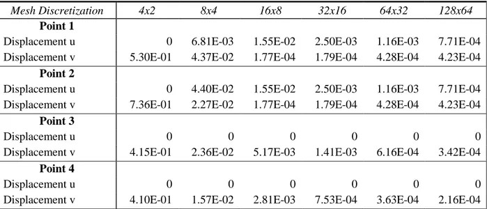
Figure 16: Medium displacement errors for a regular mesh (left side) and irregular mesh (right side): a)displacement u b) displacement v. Logarithmic scales. ... 69

Figure 17: Medium stress errors for a regular mesh (left side) and irregular mesh (right side): a) 𝜎𝑥𝑥b) 𝜎𝑥𝑦. Logarithmic scales. ... 70

Figure 18: Position on the beam of the analyzed points. ... 70

Figure 19: Model of the cantilever beam on study [28]. ... 73

Figure 20: Robutsness study of the cantilever beam for the different formulations. ... 76

Figure 21: Natural vibration frequencies: regular mesh (left-side) and irregular mesh (right-side). a) first mode b) second mode c) third mode. 77 Figure 22: First three vibration modes of the cantilever beam. ... 78

Figure 23: Vertical displacement for the cantilever beam measured on point 𝐴(𝐿, 𝐷2)... 79

Figure 24: Vertical displacement on point A using different methods (FEM). ... 80

Figure 25: Vertical displacement on point A using different methods (RPIM). ... 80

Figure 26: Vertical displacement on point A using different methods (NNRPIM). ... 80 Figure 27: Vertical displacement of point A for the cantilever beam subjected to a harmonic

(18)

Figure 29: First two vibration modes for the simply supported sandwich beam. ... 84

Figure 30: Sandwich beam with sinusoidal corrugated core along its length [66]... 86

Figure 31: Scheme of the three point bending for the sandwich beam with corrugated core [66]. ... 86

Figure 32: Sandwich beam with three layers of sinusoidal corrugated core. ... 88

Figure 33: First vibrations modes for the corrugated beam under different boundary conditions. ... 94

Figure 34: Vertical deflection for the corrugated core beam with one layer and C-C boundary conditions. ... 96

Figure 35: Scheme of the laminated plate, with two sides clamped and two sides free. ... 100

Figure 36: Representation of the harmonic solicitation. ... 101

Figure 37: Vertical displacement /m, for the laminated plate on point A. ... 102

Figure 38: Vertical displacement /m, for the laminated plate on point B. ... 102

Figure 39: Geometry of the 2D interior acoustic car [69]. ... 106

Figure 40: Geometric properties of the coupled system [70]. ... 107

Figure 41: First natural vibration mode for the uncoupled rigid fluid cavity (𝜔 = 1068 𝑟𝑎𝑑/𝑠) filled with air. ... 109

Figure 42: Second natural vibration mode for the uncoupled rigid fluid cavity (𝜔 = 1068 𝑟𝑎𝑑/𝑠) filled with air. ... 109

Figure 43: Third natural vibration mode for the uncoupled rigid fluid cavity (𝜔 = 1511 𝑟𝑎𝑑/𝑠) filled with air. ... 109

. Figure A. 1: Location of the points where the stresses were measured... 125

Figure A. 2: Location of the points where the stresses were measured for the beam with two layers. ... 137

. Figure B. 1: Vertical deflection for the corrugated core beam with one layer and C-F boundary conditions. ... 161

Figure B. 2: Vertical deflection for the corrugated core beam with one layer and C-H boundary conditions. ... 161

Figure B. 3: Vertical deflection for the corrugated core beam with one layer and H-H boundary conditions. ... 161

Figure B. 4: Vertical deflection for the corrugated core beam with two layers and C-C boundary conditions. ... 169

Figure B. 5: Vertical deflection for the corrugated core beam with two layers and C-F boundary conditions. ... 169 Figure B. 6: Vertical deflection for the corrugated core beam with two layers and C-H

(19)

Figure C. 2: Vertical deflection for the corrugated core plate with one layer and C-F boundary conditions. ... 174 Figure C. 3: Vertical deflection for the corrugated core plate with one layer and C-H boundary conditions. ... 174 Figure C. 4: Vertical deflection for the corrugated core plate with one layer and H-H boundary conditions. ... 174 Figure C. 5: Vertical deflection for the corrugated core plate with two layers and C-C boundary conditions. ... 176 Figure C. 6: Vertical deflection for the corrugated core plate with two layers and C-F boundary conditions. ... 177 Figure C. 7: Vertical deflection for the corrugated core plate with two layers and C-H boundary conditions. ... 177 Figure C. 8: Vertical deflection for the corrugated core plate with two layers and H-H boundary conditions. ... 177

(20)

(21)

List of Tables

Table 1: Punctual displacement errors using a regular mesh and FEM formulation. ... 71 Table 2: Punctual displacement errors using a regular mesh and RPIM formulation. ... 71 Table 3: Punctual displacement errors using a regular mesh and NNRPIM formulation. ... 71 Table 4: Relative frequency error: polynomial basis with one monomial and 𝑐 = 1.42 and 𝑝 = 1.03. ... 74 Table 5: Relative frequency error: polynomial basis with one monomial and 𝑐 = 0.0001 and 𝑝 = 0.999. ... 74 Table 6: Relative frequency error: polynomial basis with three monomials and 𝑐 = 1.42 and 𝑝 = 1.03. ... 75 Table 7: Relative frequency error: polynomial basis with three monomials and 𝑐 = 0.0001 and 𝑝 = 0.9999. ... 75 Table 8: Relative frequency error for the NNRPIM formulation for 𝑐 = 1.42 and 𝑝 = 1.03. ... 75 Table 9: Relative frequency error for the NNRPIM formulation for 𝑐 = 0.0001 and 𝑝 = 0.9999. ... 76 Table 10: Geometric and material properties of the sandwich beam subjected to different boundary conditions. ... 82 Table 11: First four natural frequencies (Hz) for the sandwich beam with different boundary conditions. ... 82 Table 12: Geometric and material properties of the sandwich beam subjected to different length-thickness ratios. ... 83 Table 13: Non-dimensional natural frequencies for the sandwich beam with varying 𝜆 = 𝐿𝐻 (FEM). ... 83 Table 14: Non-dimensional natural frequencies for the sandwich beam with varying 𝜆 = 𝐿𝐻 (RPIM). ... 83 Table 15: Non-dimensional natural frequencies for the sandwich beam with varying 𝜆 = 𝐿𝐻 (NNRPIM). ... 84 Table 16: Geometric and material properties of the sandwich beam with sinusoidal corrugated core. ... 86 Table 17: Maximum relative deflection, 𝑤𝑚𝑎𝑥, for the sandwich beam under three point bending. ... 87 Table 18: Relative deflection, 𝑤 , for the corrugated core beam with 2 layers under punctual load (FEM). ... 88 Table 19: Relative deflection, 𝑤 , for the corrugated core beam with 2 layers under punctual load (RPIM). ... 89 Table 20: Relative deflection, 𝑤 , for the corrugated core beam with 2 layers under distributed load (FEM). ... 89 Table 21: Relative deflection, 𝑤 , for the corrugated core beam with 2 layers under distributed

(22)

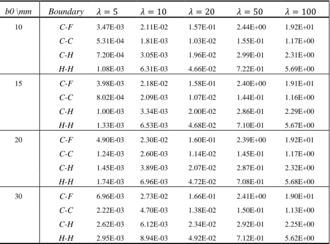
Table 22: Fundamental natural frequency (Hz) for the beam with one sinusoidal core (FEM). ... 91 Table 23: Fundamental natural frequency (Hz) for the beam with one sinusoidal core (RPIM). ... 92 Table 24: First natural frequency (Hz) for the beam with one sinusoidal core (NNRPIM). .... 93 Table 25: Relative deflection, 𝑤 , for the corrugated core beam under a harmonic distributed load (FEM). ... 95 Table 26: Relative deflection, 𝑤 , for the corrugated core beam under a harmonic distributed load (RPIM). ... 96 Table 27: Relative deflection, 𝑤 , for the corrugated core beam under a harmonic distributed load (NNRPIM). ... 96 Table 28: Relative deflection, 𝑤 , for the corrugated core plate under a harmonic distributed load (FEM). ... 98 Table 29: Relative deflection, 𝑤 , for the corrugated core plate under a harmonic distributed load (RPIM). ... 98 Table 30: Relative deflection, 𝑤 , for the corrugated core plate under a harmonic distributed load (NNRPIM). ... 99 Table 31: Geometric and material properties of the laminated plate. ... 100 Table 32: First 10 natural frequencies /Hz for the laminated plate (mesh-1). ... 100 Table 33: First 10 natural frequencies /Hz for the laminated plate (mesh-2). ... 101 Table 34: Stresses /MPa for the laminated plate, point A. ... 102 Table 35: Stresses /MPa for the laminated plate, point A1. ... 103 Table 36: Stresses /MPa for the laminated plate, point B. ... 103 Table 37: Stresses /MPa for the laminated plate, point B1. ... 103 Table 38: First 10 natural frequencies /Hz for the acoustic tube. ... 105 Table 39: First 8 natural frequencies /Hz for the 2D Car. ... 106 Table 40: Physical properties of the structure and fluid of the coupled vibro-acoustic system. ... 107 Table 41: Ten first eigenvalues /𝑟𝑎𝑑𝑠 − 1 of the coupled fluid-structure cavity filled with air. ... 108 Table 42: Ten first eigenvalues /𝑟𝑎𝑑𝑠 − 1 of the coupled fluid-structure cavity filled with water. ... 108

.

Table A. 1: Relative deflection, 𝑤 , for the corrugated core beam under punctual load (FEM). ... 122 Table A. 2: Relative deflection, 𝑤 , for the corrugated core beam under punctual load (RPIM).

(23)

Table A. 5: Relative deflection, 𝑤 , for the corrugated core beam under a distributed load (RPIM). ... 124 Table A. 6: Relative deflection, 𝑤 , for the corrugated core beam under a distributed load (NNRPIM). ... 124 Table A. 7: Stress values \MPa, for the corrugated core beam under a punctual load and C-C boundary conditions (FEM)... 125 Table A. 8: Stress values \MPa, for the corrugated core beam under a punctual load and C-F boundary conditions (FEM)... 126 Table A. 9: Stress values \MPa, for the corrugated core beam under a punctual load and C-H boundary conditions (FEM)... 126 Table A. 10: Stress values \MPa, for the corrugated core beam under a punctual load and H-H boundary conditions (FEM)... 127 Table A. 11: Stress values \MPa, for the corrugated core beam under a punctual load and C-C boundary conditions (RPIM). ... 127 Table A. 12: Stress values \MPa, for the corrugated core beam under a punctual load and C-F boundary conditions (RPIM). ... 128 Table A. 13: Stress values \MPa, for the corrugated core beam under a punctual load and C-H boundary conditions (RPIM). ... 128 Table A. 14: Stress values \MPa, for the corrugated core beam under a punctual load and H-H boundary conditions (RPIM). ... 129 Table A. 15: Stress values \MPa, for the corrugated core beam under a punctual load and C-C boundary conditions (NNRPIM). ... 129 Table A. 16: Stress values \MPa, for the corrugated core beam under a punctual load and C-F boundary conditions (NNRPIM). ... 130 Table A. 17: Stress values \MPa, for the corrugated core beam under a punctual load and C-H boundary conditions (NNRPIM). ... 130 Table A. 18: Stress values \MPa, for the corrugated core beam under a punctual load and H-H boundary conditions (NNRPIM). ... 130 Table A. 19: Stress values \MPa, for the corrugated core beam under a distributed load and C-C boundary conditions (FEM). ... 131 Table A. 20: Stress values \MPa, for the corrugated core beam under a distributed load and C-F boundary conditions (C-FEM). ... 131 Table A. 21: Stress values \MPa, for the corrugated core beam under a distributed load and C-H boundary conditions (FEM). ... 132 Table A. 22: Stress values \MPa, for the corrugated core beam under a distributed load and H-H boundary conditions (FEM). ... 132 Table A. 23: Stress values \MPa, for the corrugated core beam under a distributed load and C-C boundary conditions (RPIM). ... 133 Table A. 24: Stress values \MPa, for the corrugated core beam under a distributed load and C-F boundary conditions (RPIM). ... 133 Table A. 25: Stress values \MPa, for the corrugated core beam under a distributed load and

(24)

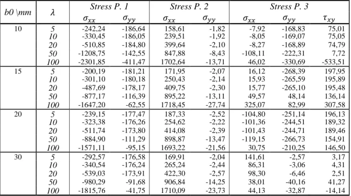
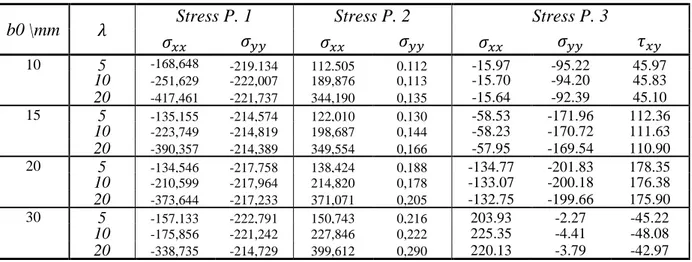
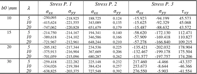
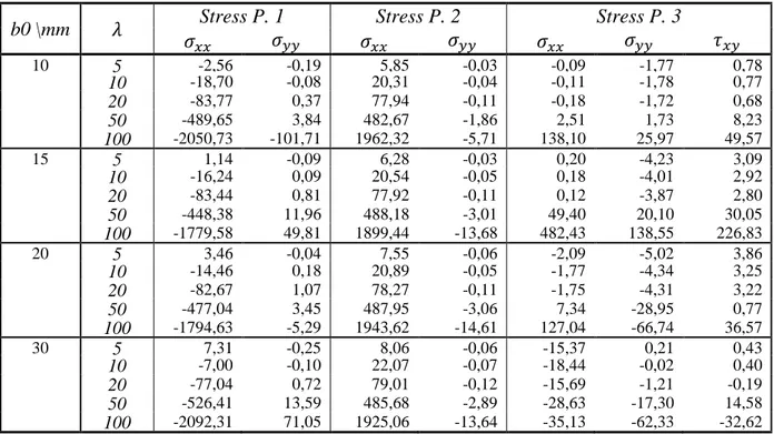
C-Table A. 26: Stress values \MPa, for the corrugated core beam under a distributed load and H-H boundary conditions (RPIM). ... 134 Table A. 27: Stress values \MPa, for the corrugated core beam under a distributed load and C-C boundary conditions (NNRPIM)... 135 Table A. 28: Stress values \MPa, for the corrugated core beam under a distributed load and C-F boundary conditions (NNRPIM). ... 135 Table A. 29: Stress values \MPa, for the corrugated core beam under a distributed load and C-H boundary conditions (NNRPIM). ... 135 Table A. 30: Stress values \MPa, for the corrugated core beam under a distributed load and H-H boundary conditions (NNRPIM). ... 136 Table A. 31: Stress values \MPa, for the 2 layers beam under a punctual load and C-C boundary conditions (FEM)... 137 Table A. 32: Stress values \MPa, for the 2 layers beam under a punctual load and C-F boundary conditions (FEM)... 138 Table A. 33: Stress values \MPa, for the 2 layers beam under a punctual load and C-H boundary conditions (FEM)... 139 Table A. 34: Stress values \MPa, for the 2 layers beam under a punctual load and H-H boundary conditions (FEM)... 140 Table A. 35: Stress values \MPa, for the 2 layers beam under a punctual load and C-C boundary conditions (RPIM). ... 141 Table A. 36: Stress values \MPa, for the 2 layers beam under a punctual load and C-F boundary conditions (RPIM). ... 142 Table A. 37: Stress values \MPa, for the 2 layers beam under a punctual load and C-H boundary conditions (RPIM). ... 143 Table A. 38: Stress values \MPa, for the 2 layers beam under a punctual load and H-H boundary conditions (RPIM). ... 144 Table A. 39: Stress values \MPa, for the 2 layers beam under a distributed load and C-C boundary conditions (FEM)... 145 Table A. 40: Stress values \MPa, for the 2 layers beam under a distributed load and C-F boundary conditions (FEM)... 146 Table A. 41: Stress values \MPa, for the 2 layers beam under a distributed load and C-H boundary conditions (FEM)... 147 Table A. 42: Stress values \MPa, for the 2 layers beam under a distributed load and H-H boundary conditions (FEM)... 148 Table A. 43: Stress values \MPa, for the 2 layers beam under a distributed load and C-C boundary conditions (RPIM). ... 149 Table A. 44: Stress values \MPa, for the 2 layers beam under a distributed load and C-H

(25)

Table B. 2: Third natural frequency (Hz) for the beam with one sinusoidal core (FEM). ... 155 Table B. 3: Second natural frequency (Hz) for the beam with one sinusoidal core (RPIM). 156 Table B. 4: Third natural frequency (Hz) for the beam with one sinusoidal core (RPIM). ... 157 Table B. 5: Second natural frequency (Hz) for the beam with one sinusoidal core (NNRPIM). ... 158 Table B. 6: Third natural frequency (Hz) for the beam with one sinusoidal core (NNRPIM). ... 159 Table B. 7: Maximum absolute stresses for the beam with 1 layer (FEM). ... 159 Table B. 8: Maximum absolute stresses for the beam with 1 layer (RPIM). ... 160 Table B. 9: Maximum absolute stresses for the beam with 1 layer (NNRPIM)... 160 Table B. 10: Fundamental natural frequency (Hz) for the beam with two sinusoidal cores (FEM). ... 162 Table B. 11: Second natural frequency (Hz) for the beam with two sinusoidal cores (FEM). ... 163 Table B. 12: Third natural frequency (Hz) for the beam with two sinusoidal cores (FEM). . 164 Table B. 13: Fundamental natural frequency (Hz) for the beam with two sinusoidal cores (RPIM). ... 165 Table B. 14: Second natural frequency (Hz) for the beam with two sinusoidal cores (RPIM). ... 166 Table B. 15: Third natural frequency (Hz) for the beam with two sinusoidal cores (RPIM). 167 Table B. 16: Maximum absolute stresses for the beam with 2 layers (FEM). ... 167 Table B. 17: Maximum absolute stresses for the beam with 2 layers (RPIM). ... 168 Table B. 18: Maximum absolute stresses for the beam with 2 layers (NNRPIM). ... 168

..

Table C. 1: Maximum absolute stresses for the plate with 1 layer (FEM). ... 172 Table C. 2: Maximum absolute stresses for the plate with 1 layer (RPIM). ... 172 Table C. 3: Maximum absolute stresses for the plate with 1 layer (NNRPIM). ... 173 Table C. 4: Maximum absolute stresses for the plate with 2 layers (FEM). ... 175 Table C. 5: Maximum absolute stresses for the plate with 2 layers (RPIM). ... 175 Table C. 6: Maximum absolute stresses for the plate with 2 layers (NNRPIM). ... 176

(26)

(27)

1. Introduction

The resources and time spent on the experimental analysis of the dynamic behavior of structures and other physical phenomenon can have an exponential increase when dealing with complex geometries and materials. In recent decades, a significant effort has been applied on the development of numerical computational tools that simulate the behavior of systems under different solicitations. Although, frequently, this methods do not present a good correlation when compared to experimental results [1]. One scientific field that has been attracting recent attention is the field of vibro-acoustics. The need to optimize the vibratory response of structures on areas like aeronautics and aerospace can be a major factor for competitiveness in the industry.

Discrete numerical methods, such as the FEM, have been extended to the acoustical formulation. Although, despite being the most popular method, it can prove to be inefficient some times for vibro-acoustic problems, showcasing difficulties in correctly simulating the wave propagations [2]. Other numerical techniques, like the meshless methods, have gained popularity over the last few years, mainly for being able to solve some difficulties associated with FEM when denser nodal zones are required.

In this work, the weak formulation of acoustical problems is extended to two different meshless methods, the RPIM (Radial Point Interpolation Method) and NNRPIM (Natural Neighbor Radial Point Interpolation Method). Several dynamic analysis (free, forced vibrations and vibro-acoustics) are performed and compared with the results displayed by the finite element method and also compared with the available results documented in literature.

(28)

1.1 Acoustic

The study of an acoustic problem can be breakdown to the interaction between a fluid inducing pressure over a vibrating structure and vice-versa. To characterize the behavior of the structure, the coupling with the surrounding fluid and the boundary conditions must be taken into account, which will vary with both geometry and properties of the fluid and structure.

The analysis of the coupled system can be divided in three particular cases: interior problems, where the fluid is encased inside the structure; exterior problems, where the fluid domain surrounds the structures; interior/exterior problems, which is a combination of both problems. Besides this division, in acoustic problems the frequency domain must also be taken into consideration, since it will define the approach that must be considered when solving the coupled problem. The system can be working in low, mid (MF) and high frequencies (HF) - Figure 1.

Figure 1: Typical FRF (Frequency Response Function) of a vibroacoustic system [3].

In the low frequencies domain, the resonances are well spaced, corresponding to a modal-controlled behavior. For this case, FEM or BEM solutions [3] usually present accurate results to describe the response of the coupled system.

In the high frequencies domain, the response no longer has visible resonance of local strong variations, implying that the modal density of the system is uniform, thus the number of modes present is high. For acoustic problems under this domain, generally statistical energy analysis (SEA) [4] is the best approach.

On the intermediate domain (mid-frequencies) both low and high frequency behaviors can be found, for which hybrid deterministic-statistical methods are usually applied in solving the system [5].

For an acoustic pressure disturbance 𝑝(𝒙, 𝑡) in a perfect fluid of volume Ω_f, being 𝜌₀ the density and 𝑐₀ the sound speed on the fluid, the inhomogeneous wave equation, also known as

(29)

the frequency range increases. For instance, methods like the FE still cannot be fully applied to solve this systems due to problems from the pollution error [7] that arises from the dispersive nature of the numerical wave.

To try and eliminate this dispersion, many numerical methods have been proposed. The first idea was to stabilize the finite element method [8, 9], but at the end it was shown that such technique did not enhanced significantly the FEM. Next, higher order approximations based on the hp formulation [10] and meshless approaches [11] were proposed.

Bouillar et al. [12] applied the EFGM to the acoustic field, but concluded that this meshless method is still affected by pollution errors, even though in a much lesser magnitude compared to the FEM. An improved method for the EFGM was proposed [13]. Interpolator methods were later tested, with the RPIM being used to study the dispersion effect in 2D acoustic problems [14], showing that such method can significantly reduce the dispersion error. Adaptations to the RPIM were proposed, like the linearly conformed Radial Point Interpolation Method (LC-RPIM) [15], the edge-based smoothed Point Interpolation Method (ES-PIM) [16], the cell-based smoothed Radial Point Interpolation Method (CS-RPIM) [17], and others.

In both cases, there were still documented problems arising from the pollution error, and that may be the reason for the inexistence of efficient discrete numerical methods for the medium frequency range on acoustical problems [18].

Thus, the principal interest of this work lies in the analysis of the behavior and accuracy of two different meshless methods on the acoustical study of coupled fluid-structure problems.

(30)

1.2 Meshless Methods

In past decades, the finite element method (FEM) has been used in a wide range of engineering applications. It is a numerical method best used to solve problems with complex geometries and/or boundary conditions, since it is based on the subdivision of the initial geometry into small domains called elements. The association of these elements forms a mesh that assures nodal connectivity for all the structure. [19]

Despite the popularity and competence of the FEM, meshless methods have been seek with increase interest over the last few years as an efficient technique for numerically solving partial differential equations. Since it does not relies on a mesh, such as the case of the FEM, this formulation becomes more suitable for solving problems with complex geometries where mesh construction could represent a computational burdensome task [20].

Comparing both methods, meshless formulations presents some major advantages, being more appropriated for solving problems with moving discontinuities like crack propagation, more capable of handling large deformations (it is simpler to incorporate h-adaptivity), having higher-order continuous shape functions, non-local interpolation features and no mesh alignment sensitivity. As drawbacks, besides the higher computational costs, the shape functions require high-order integration schemes in order to be correctly computed, also for some formulations imposing essential boundary conditions can be troublesome [21].

In meshless methods, the geometry is discretized in nodes arbitrarily distributed along the domain, and instead of using elements, the field functions are approximated within “influence-domains” set for each interest point [22]. The first works on this method date back to the seventies with the Smooth Particle Hydrodynamics (SPH) methods [23], using kernel estimates to solve problems involving fluid masses moving arbitrarily in the absence of boundaries [24]. This method gave origin to the Reproducing Kernel Particle Method (RKPM) [25].

Later on, new approaches provided significant progress to the meshless method. Starting with the Diffuse Element Method (DEM), that uses moving least-square approximations in the Galerkin formulation, this way replacing the FEM interpolation, valid on an element, with a local weighted least squares fitting, valid in a small neighborhood of an arbitrary point “x” [26]. Belytschko gave significant improvements on the DEM, creating its own method called the Element-Free Galerkin Method (EFGM) [27].

Meshless methods can be divided in two categories depending on the used formulation, which can be either the strong-form or the weak-form. The first seeks the direct resolution of the partial differential equations ruling the studied problem. The weak-form uses a variational principle in order to minimize the residual weight of the differential equations, to do that the method replaces the exact solution with an approximated function affected by a test function [28].

Girault, Kao & Perrone and Liszka [29-31] gave significant contributions in the development of the global strong-form formulation for meshless methods, such as the General Finite Difference Method (GFDM). Later works on this formulation involve the Finite Point Method

(31)

MSL are instances of partitions of unity, which lead to significant improvements on these methods. Another class of meshless methods are based on the local weak form, that are generated on overlapping subdomains, instead of using a global weak form [21]. For example, the Meshless Free Petrov-Galerkin (MLPG) [38], initially used for solving linear and nonlinear potential problems, later evolved into the Method of Finite Spheres (MFS) [39]. Due to the complexity on computing the shape function and their derivatives, and the lack of the Kronecker delta property, which arises problems when essential and natural boundary conditions are to be imposed, several interpolant meshless methods were developed. Liu initially proposed the Point Assembly Method (PAM) [40] and the Point Interpolation Method (PIM) [41], the later demonstrating some singularity problems for regular nodal distributions. The Radial Point Interpolation Method (RPIM) [42] was then introduced to avoid such problems, relying on the use of radial basis functions, mainly the multi-quadrics (MQ) functions [43]. Other relevant interpolant meshless methods are the Meshless Finite Element Method (MFEM) [44] and the Natural Element Method (NEM) [45]. Recently, Belinha combined both the NEM and RPIM formulations, giving origin to the Natural Neighbour Radial Point Interpolation Method (NNRPIM) [46]. This last method uses the concepts of influence-cell, such as the Voronoї diagrams [47] and the Delaunay tessellation to construct the integration mesh and influence domains of each node.

Both the RPIM and NNRPIM use radial interpolation functions, possessing the delta Kronecker and compact support properties. These methods differ in the way the nodal connectivity is imposed. On the RPIM, the nodal connectivity is established by the overlapping of the “influence-domains”, and thus, requires the use of a background integration mesh to allocate the integrations points, being nodal independent.

On the other hand, the recently developed NNRPIM uses the concept of “influence-cells”, relying on mathematical methods such as the Voronoї diagrams and Delaunay tessellation. Thus, for the distribution of the integration points, only the spatial position of the nodes is necessary, making the NNRPIM a truly meshless method, whose integration scheme is nodal dependent.

Despite being a recent method, the NNRPIM has already been applied in many different fields: in the static analysis of isotropic and orthotropic plates [48], nonlinear problems [49], crack opening problems [50], bone tissue remodeling [28] and others.

In the present work, the FEM, RPIM and NNRPIM formulations are used to solve the diverse numerical examples of static, free and forced vibrations and vibro-acoustic problems. For the NNRPIM, it is the first time this method is applied to the analysis of acoustical problems.

(32)

1.3 Thesis Objectives

This thesis aims to analyze of the performance of two meshless methods, the RPIM and NNRPIM, on the prediction of the behavior of structures and coupled fluid-structures problems under dynamic loads.

For this matter, a sequence of MATAB® algorithms will be created. These consists on algorithms that permit the study of free and forced vibrations on 2D and 3D problems as well as the acoustical study of uncoupled and interior coupled fluid-structure problems.

As a final result, for the free and forced vibrations studies, these algorithms must be able to:  Solve eigenvalue problems and plot the normalized eigenvectors of the problem;  Calculate the nodal dynamic displacements for any given load and damping present in

the system;

 Calculate the dynamic stresses and strains at each integration point;  Plot the dynamic displacement at any given point in time;

 Plot the displacement of any node along the time domain;

 For harmonic loads, plot the displacement of any node along the frequency domain; For the acoustical algorithms, they must be able to:

 Solve eigenvalue problems and plot the normalized eigenvectors of the Helmholtz equation;

 Calculate the nodal pressure for uncoupled acoustical problems;

 Solve eigenvalue problems and plot the normalized eigenvectors of the interior coupled problem;

 Calculate the nodal pressure for the fluid and nodal displacements for the structure for an interior coupled problem;

 Plot of the displacements (for the structure) and pressure (for the fluid) of any node along the frequency domain;

 Calculation of acoustic parameters;

For the developed software, both task must be able to be performed on both the FEM, RPIM and NNRPIM formulations.

After the creation of the algorithms, examples consisting mainly in laminated and sandwich beams and plates will be solved and their results compared for both formulations and with the literature whenever possible.

(33)

1.4 Thesis Arrangement

This thesis is divided into 9 chapters: Introduction, Meshless Methods, Solid Mechanics, Plane Elasticity, Vibrations, Vibro-Acoustics, Routines, Numerical Examples and Conclusions.

In the first chapter, an overview of the topics presented in the thesis is given. Explaining the development of the meshless methods, forced vibrations and the acoustical formulation In the next five chapters is provided a detailed explanation of the theoretical formulations used on the thesis.

In chapter 7. Routines, an explanation of the computed algorithms is given. In this chapter its possible to understand the code that the MATLAB® software runs in order to obtain the desired results.

In chapter 8, are described several numerical examples run with both formulations using the created algorithms. When possible, the results are compared with the theoretical solutions and other results present in the literature.

In the last chapter, the main conclusions about this work are discussed, retaining also some possibilities and recommendations for future works on the subject.

(34)

(35)

2. Meshless Methods

Meshless methods follow a general procedure: define the nodal mesh that discretizes the geometry; construct the background mesh constituted by the integration points; establish the influence domains for each integration point; creat the interpolation functions; create the local stiffness and mass matrix; assemble the local matrices into the global matrices of the problem; impose the essential and natural boundary conditions and solve the system of equations. The distribution of the nodal mesh has a direct influence in the quality and accuracy of the results. Regular meshes usually perform better than irregular meshes - Figure 2, and for problems involving stress concentrations (crack propagations, clamped boundaries, etc.) it may be necessary to have a higher nodal density around those areas to assure good results. As such, there is not an exact nodal mesh to better discretize a geometry. The choice must also take in consideration the computational costs involved in analyzing the amount of degrees of freedom chosen, and so an equilibrium between accuracy and efficiency has to be attained.

Figure 2: a) Irregular mesh; b) regular mesh [28].

It is after creating the nodal mesh that the meshless methods differ from the FEM, since no elements connecting the nodes are established. Instead, a background integration mesh is constructed. Depending on the method adopted, this background mesh can be nodal dependent (like in the case of the NNRPIM), or nodal independent (RPIM for example) - Figure 3. On truly meshless methods, the nodes are used as the integration points or used to directly define the integration points, removing the need to create a background mesh.

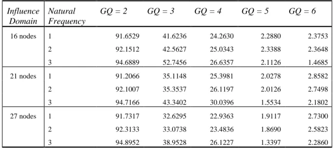
In most cases, this integration mesh is distributed having in account the Gauss-Legendre quadrature rule

(36)

After the integration mesh has been assembled the “influence-domain” for each integration point is established by generating concentric areas (or volumes for 3D cases) around this points, and every node inside belongs to the “influence-domain” of that point. Unlike the FEM, on meshless methods the nodal connectivity is imposed with the overlapping of the various influence domains.

With the “influence-domain” defined for each interest point, the shape functions and its derivatives can be calculated. This process heavily depends on the formulation used, as they can be either interpolation or approximation functions. The RPIM and NNRPIM methods are interpolator methods, meaning that the shape functions pass at every node, thus possessing the delta Kronecker property.

Next the local matrices for each integration point can be constructed and assembled into the global matrices. This process is in everything similar to the FEM, where the global matrices are obtained by allocating the local matrix in their respective degrees of freedom, that is,

𝑲 = ∑ 𝑹_𝑗𝑇 𝑁

𝑗=1

· 𝑲_𝑗∗· 𝑹𝑗 (2)

Where 𝑹_𝒋 is the allocation matrix connecting the local degrees of freedom from the local

matrix with the global degrees of freedom. The same process is applied for the mass matrix and force vector.

To impose the essential boundary conditions, the most three common methods are: the Lagrange multipliers, the direct imposition method and the penalty method [28]. Since the RPIM and NNRPIM are interpolations methods, the essential boundary conditions can be imposed using either method.

In this work an extension of the penalty method was adopted to impose the boundary conditions, where the rows and columns of the constrained degrees of freedom are removed from the global matrices, resulting in a smaller system of equations to solve and avoiding the appearance of rigid body modes when using modal superposition.

(37)

2.1 Radial Point Interpolation Method (RPIM)

As already stated, the Point Interpolation Method [41] is an efficient method to create interpolation shape functions for meshless methods possessing the Kronecker delta property. It uses polynomial basis functions to construct shape functions, forcing the interpolation function to pass through all the scattered nodes in an influence domain. Despite those advantages, the PIM may lead to singular moment matrices when creating the shape functions if the nodes are perfectly aligned.

To bypass this problem, a radial basis function was added to the PIM generic shape functions, creating the RPI shape functions [42]. However, the inclusion of these functions increases the computational costs.

Figure 4: Interpolation function 𝑢ℎ_{(𝑥) and the discrete nodal parameters (𝑥}

𝑖) [28].

It has been proved that the absence of a polynomial basis on the RPI method would lead to failure of the standard patch test, since a 𝐶1 continuity needs to be assured. Adding this polynomial basis ensures the stability of this method.

Considering an approximation function 𝑢ℎ_{(𝒙) in an influence domain, being 𝑛 the number of} nodes inside the influence domain of 𝒙𝐼. The RPIM forces the approximation function to pass through all nodal data within the influence domain, using a radial basis function 𝑟𝑖(𝒙) and a polynomial basis function 𝑝𝑗(𝒙). Thus, the interpolated value for an interest point 𝒙𝐼 can be obtained with: 𝑢ℎ(𝒙𝐼) = ∑ 𝑟𝑖(𝒙𝐼)𝑎𝑖 𝒏 𝒊=𝟏 + ∑ 𝑝𝑗(𝒙𝐼)𝑏𝑗 𝒎 𝒋=𝟏 = 𝑹𝑇(𝒙𝐼)𝒂 + 𝑷𝑇(𝒙𝐼)𝒃 (3)

where 𝑎_𝑖 and 𝑏_𝑗 are the coefficients of 𝑟_𝑖(𝒙) and 𝑝_𝑗(𝒙). The vectors can be defined as: 𝒂𝑻 _{= {𝑎}₁ _𝑎₂ _⋯ _𝑎_𝑛_} 𝒃𝑻 _{= {𝑏} 1 𝑏2 ⋯ 𝑏𝑛} 𝑹𝑻(𝒙) = [𝑟1(𝒙) 𝑟2(𝒙) ⋯ 𝑟𝑛(𝒙)] 𝑷𝑻(𝒙) = [𝑝1(𝒙) 𝑝2(𝒙) ⋯ 𝑝𝑚(𝒙)] (4)

(38)

𝑷𝑻(𝒙) = [1 𝑥 𝑦 𝑥2 _𝑥𝑦 _…] ₍₅₎ For the radial basis functions 𝑟_𝑖(𝒙_𝐼) the only variable present is the Euclidian norm between the field nodes and the considerer point 𝒙. For a three-dimensional space, this distance between an interest point 𝒙_𝐼 and another point 𝒙_𝑖 can be expressed as,

𝑑_𝐼𝑖 = ‖𝒙_𝑖 − 𝒙_𝐼‖ = √(𝑥_𝑖− 𝑥_𝐼)2_{+ (𝑦}

𝑖 − 𝑦𝐼)2+ (𝑧𝑖 − 𝑧𝐼)2 (6) There are several different RBF that can be applied on the construction of the shape functions [43], being the multi-quadratics (MQ) functions the most used: 𝑟_𝑖(𝒙_𝐼) = (𝑑_𝐼𝑖2 _{+ 𝑐}2₎𝑝_. Comprehensively, the MQ-RBF is dependent on two shape parameters, 𝑐 and 𝑝, that must be determined and optimized in order to obtain accurate results [51].

Figure 5: Triangle of Pascal [28].

In order to calculate the values of the coefficients 𝑎_𝑖 and 𝑏_𝑗 a new set of equations must be taken into consideration [52], which can be presented as:

∑ 𝑝_𝑗(𝒙) 𝑛

𝑖=1

𝑎_𝑖 = 0, 𝑗 = 1,2, … , 𝑚 (7)

Now the system with 𝑛 + 𝑚 unknowns can be solved by forcing the interpolant functions to pass through all nodes in the influence domain, expressed in matrix form as:

(39)

𝑹 = [ 𝑟1(𝒙1) 𝑟2(𝒙1) 𝑟₁(𝒙₂) 𝑟₂(𝒙₂) ⋯ 𝑟𝑛(𝒙𝑛) ⋯ 𝑟_𝑛(𝒙_𝑛) ⋮ ⋮ 𝑟₁(𝒙_𝑛) 𝑟₂(𝒙_𝑛) ⋱ ⋮ ⋯ 𝑟_𝑛(𝒙_𝑛) ] (9)

The coefficient matrix 𝑷 is,

𝑷 = [ 𝑝1(𝒙1) 𝑝2(𝒙1) 𝑝₁(𝒙₂) 𝑝₂(𝒙₂) ⋯ 𝑝𝑚(𝒙1) ⋯ 𝑝_𝑚(𝒙₂) ⋮ ⋮ 𝑝₁(𝒙_𝑛) 𝑝₂(𝒙_𝑛) ⋱ ⋮ ⋯ 𝑝_𝑚(𝒙_𝑛) ] (10)

Both matrixes are symmetrical, which means 𝑴_𝑇 is also symmetric. By inverting the total

moment matrix 𝑴𝑇, it is possible to obtain the values of the coefficients 𝑎𝑖 and 𝑏𝑗,

{𝒂

𝒃} = 𝑴𝑇−1{ 𝒖_𝑠

𝟎} (11)

Substituting back on equation (3),

𝑢ℎ(𝒙) = [𝑹𝑇_{(𝒙) 𝑷}𝑇_(𝒙)]𝑴 𝑇 −1_{𝒖𝑠

𝟎} = 𝝋𝑇(𝒙)𝒖𝑠 (12)

The matrix of shape functions is defined as,

𝝋(𝒙) = [𝜑1(𝒙) 𝜑2(𝒙) ⋯ 𝜑𝑛(𝒙)] (13)

The approximation function 𝑢ℎ_{(𝒙) is now given by,} 𝑢ℎ_{(𝒙) = ∑ 𝜑}

𝑖(𝒙) 𝑛

𝑖=1

𝑢_𝑖 (14)

For two distinct points, sharing the same 𝑛 nodes inside their influence-domain, the obtained coefficients 𝑎𝑖 and 𝑏𝑗 will be the same for both points, therefore the total moment matrix is not directly dependent on the spatial position of the considered point. The derivatives of the shape functions can be easily obtained since only the radial and polynomial basis needs to be derivate, that is,

𝜕𝑢ℎ(𝒙) 𝜕𝜉 = ∑ 𝜕𝜑_𝑖(𝒙) 𝜕𝜉 𝑢𝑖 𝑛 𝑖=1 (15)

where 𝜉 is a generic variable. The RPI shape functions enjoy a range of properties, such as consistency, reproducibility, partition of unity, compact support and the Kronecker delta property. A detailed description of RPI shape functions can be found in the literature [28].

(40)

2.2 Natural Neighbour Radial Point Interpolation Method (NNRPIM)

The NNRPIM shares many resemblances with the RPIM formulation, in which both are interpolator methods possessing the Kronecker Delta property, and use a radial basis functions to construct the shape functions. As such, after the construction of the “influence-domain” for each interest point both formulations work the same way.

Where they differ is in the imposition of the nodal connectivity and in the construction of the background integration mesh. Here the NNRPIM uses the concept of “influence-cell” to draw the “influence-domain” for each interest point. The method relies on the use of geometrical concepts such as the Voronoї diagrams and the Delaunay tessellations.

To obtain the Voronoї diagram for each node the mathematical concept of natural neighbor is used [53]. This method consists in finding the closest subset of nodes for a given point and giving to each node a weight based on its proportional area. As a result, the Voronoї cell for each node consist in the aggregate of all points that are more close to the considered node than to any other node on the structure.

In Figure 6 is illustrated the construction of a Voronoї cell, region 𝑉₀. For the considered point, 𝑛0, a straight line is drawn from this node to the closest node. Next, a line normal to this one is drawn on the closest node, and every point on the other side of this line is rejected. This process is then repeated until all normal lines form a closed geometry, from this point all neighbor nodes have been found, which correspond to the nodes on the lines.

After the neighbor nodes are found, the Voronoї cell for 𝑛₀ is obtained dividing the distance to each node by half, that is, the Voronoї cell is the homothetic form of the closed geometry, being

𝑑_0𝑖∗ = ‖𝑥0− 𝑥𝑖‖

(41)

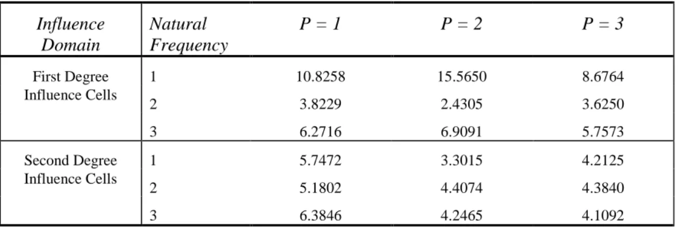
After applying this methodology to every node on the structure, the influence cell concept can be used to construct the “influence-domain” for each interest point. There are mainly two degrees of influence cell used: “first degree influence-cell” - where the neighbor nodes of a point of interest are considered - and “second degree influence-cell” - where the natural neighbor nodes of the neighbor nodes of a point of interest are considered on the influence-cell - Figure 7.

Figure 7: a) First degree influence-cell b) second degree influence cell [28].

To impose the background integration mesh, a nodal based integration scheme is used. Here, the Voronoї cells are divided into small areas, either quandrangular (for irregular meshes) or triangular (for regular meshes). Each of these areas is then populated with Gauss Points, depending on the desired quadrature. The integration weight of each integration point is given by

𝜔𝐼 = 𝜔𝜉· 𝜔𝜂· ( 𝐴

4) (17)

Where 𝐴 is the area of the respective sub-quadrilateral and 𝜔̅̅̅̅ and 𝜔𝜉 ̅̅̅̅ are the integration 𝜂 weights given by the Gauss-Legendre Quadrature. In Figure 8 is illustrated how to divide the cells into small areas, and the small shapes obtained from the division with one gauss point.

(42)

(43)

(44)

3.1 Stress and Strain Fields

Consider a 3D solid structure. At any given point of the structure the stress and strain fields are defined as:

𝝈 = {𝜎𝑥 𝜎𝑦 𝜎𝑧 𝜏𝑥𝑦 𝜏𝑦𝑧 𝜏𝑧𝑥}𝑇 (18)

𝜺 = {𝜀𝑥 𝜀𝑦 𝜀𝑧 𝛾𝑥𝑦 𝛾𝑦𝑧 𝛾𝑧𝑥}𝑇 (19)

The strain components can be directly obtained from the displacement field. Denoting the components 𝑢, 𝑣 and 𝑤 as the displacements along the 𝑥, 𝑦 and 𝑧 axis, the strain field can be calculated using the following expressions

𝜀_𝑥 =𝜕𝑢 𝜕𝑥 ; 𝜀𝑦 = 𝜕𝑣 𝜕𝑦 ; 𝜀𝑧= 𝜕𝑤 𝜕𝑧 𝛾_𝑥𝑦= 𝜕𝑢 𝜕𝑦+ 𝑑𝑣 𝑑𝑥 ; 𝛾𝑥𝑧 = 𝜕𝑢 𝜕𝑧+ 𝑑𝑤 𝑑𝑥 ; 𝛾𝑦𝑧 = 𝜕𝑣 𝜕𝑧+ 𝑑𝑤 𝑑𝑦 (20)

And the stress tensor is calculated multiplying the constitutive matrix, 𝑫, defined by material properties of the structure, with the strain tensor, resulting

𝝈 = 𝑫𝜺 (21)

If initial stresses or strains are to be considered, then, expression (21) becomes,

𝝈 = 𝑫(𝜺 − 𝜺0) + 𝝈0 (22)

The equilibrium equations for the static analysis of a general 3D problem are 𝜕𝜎_𝑥 𝜕𝑥 + 𝜕𝜏_𝑥𝑦 𝜕𝑦 + 𝜕𝜏_𝑥𝑧 𝜕𝑥 + 𝑓𝑥 = 0 𝜕𝜏_𝑥𝑦 𝜕𝑥 + 𝜕𝜎_𝑦 𝜕𝑦 + 𝜕𝜏_𝑦𝑧 𝜕𝑧 + 𝑓𝑦 = 0 𝜕𝜏_𝑥𝑧 𝜕𝑥 + 𝜕𝜏_𝑦𝑧 𝜕𝑦 + 𝜕𝜎_𝑧 𝜕𝑧 + 𝑓𝑧 = 0 (23) Or in matrix form 𝑳𝝈 + 𝒇 = 0 (24)

(45)

3.2 Strong and Weak Form Formulations

In the strong form formulations, a solution is seek at every single point of the structure, which means that the equations governing the strong form must be satisfied for any point in the considered global domain. For complex geometries and boundary conditions, a solution to the differential system equations governing the studied phenomenon may not always be possible to attain.

In those cases, a weak form formulation is often sought. Here, the differential system equations no longer needs to be valid at every point on the structure, but instead is established at discrete points spread across the domain. The implementation of boundary conditions is also simple, since they can be directly applied on an arbitrary node. As a downside, this approximation means the accuracy of the solution is dependent on the number of points discretizing the problem domain.

(46)

3.2.1 Weak Form of Galerkin

The Galerkin form is a variational principle that is based on the energy principle - the Hamilton’s principle.

The Hamilton’s principle states that: “of all admissible displacements configurations satisfying the compatibility conditions, the essential boundary conditions and the initial and final time conditions, the real solution correspondent configuration is the one which minimizes the Lagrangian functional L” [28].

𝐿 = 𝑇 − 𝑈 + 𝑊_𝑓 (25)

where 𝑇 is the kinetic energy, 𝑈 is the strain energy and 𝑊_𝑓 is the work produced by the external forces. For a solid domain with volume Ω, being 𝒖 and 𝒖̇ the displacement and velocity fields, the kinetic energy is define by,

𝑇 =1 2∫ 𝜌𝒖̇

𝑇_{𝒖̇ 𝑑Ω} Ω

(26) being 𝜌 the solid’s mass density. For elastic materials, the strain energy is defined as,

𝑈 =1

2∫ 𝜺 𝑇 Ω

𝝈 𝑑Ω (27)

being 𝜺 and 𝝈 the strain and stress vectors respectively. The work produced by the external forces can be given by,

𝑊_𝑓= ∫ 𝒖𝑇_{𝒃 𝑑Ω + ∫ 𝒖}𝑇_{𝒕 𝑑Γ} Γ

Ω

(28) being 𝒃 body forces and Γ the traction boundary where the external forces 𝒕 are applied. Thus, the Hamilton’s principle can be written as,

𝛿 ∫ [1 2∫ 𝜌𝒖̇ 𝑇_{𝒖̇ 𝑑Ω} Ω −1 2∫ 𝜺 𝑇 Ω 𝝈 𝑑Ω + ∫ 𝒖𝑇𝒃 𝑑Ω + ∫ 𝒖𝑇𝒕 𝑑Γ Γ Ω ] 𝑡2 𝑡1 𝑑𝑡 = 0 (29)

Moving the variation operator 𝛿 to inside the integral results,

∫ [1 2∫ 𝛿 (𝜌𝒖̇ 𝑇_{𝒖̇) 𝑑Ω} Ω −1 2∫ 𝛿(𝜺 𝑇 Ω 𝝈) 𝑑Ω + ∫ 𝛿𝒖𝑇𝒃 𝑑Ω + ∫ 𝛿𝒖𝑇𝒕 𝑑Γ Γ Ω ] 𝑡2 𝑡1 𝑑𝑡 = 0 (30) Using the chain rule variation and the scalar property, that is

∫ 𝛿(𝒖𝑇𝒖) 𝑑𝑡 𝑡2 𝑡1 = ∫ (𝛿𝒖𝑇 𝑡2 𝑡1 𝒖 + 𝒖𝑇𝛿𝒖) 𝑑𝑡 = 2 ∫ (𝛿𝒖𝑇𝒖) 𝑑𝑡 𝑡2 𝑡1 (31) and integrating by parts, the first term of equation (29) becomes,

∫ [1 2∫ 𝛿 (𝜌𝒖̇ 𝑇_{𝒖̇) 𝑑Ω} Ω ] 𝑡2 𝑡1 𝑑𝑡 = − ∫ [𝜌 ∫ 𝛿 (𝜌𝒖𝑇𝒖̈) 𝑑Ω Ω ] 𝑡2 𝑡1 (32)

(47)

Therefore, the second term becomes, ∫ [1 2∫ 𝛿 (𝜺 𝑇_{𝝈) 𝑑Ω} Ω ] 𝑡2 𝑡1 𝑑𝑡 = ∫ [∫ 𝛿 𝜺𝑇𝝈 𝑑Ω Ω ] 𝑑𝑡 𝑡2 𝑡1 (34) The Hamilton’s principle now becomes,

∫ [−𝜌 ∫ 𝛿 (𝒖𝑇𝒖̈) 𝑑Ω Ω − ∫ 𝛿 𝜺𝑇𝝈 𝑑Ω Ω + ∫ 𝛿𝒖𝑇𝒃 𝑑Ω + ∫ 𝛿𝒖𝑇𝒕 𝑑Γ Γ Ω ] 𝑑𝑡 = 0 𝑡2 𝑡1 (35) In order for the equation to be zero at any given time, the integrand must be null, leading to what is known as the ‘Galerkin weak form’, or the principle of virtual work,

−𝜌 ∫ 𝛿 (𝒖𝑇_{𝒖̈) 𝑑Ω} Ω − ∫ 𝛿 𝜺𝑇_{𝝈 𝑑Ω} Ω + ∫ 𝛿𝒖𝑇_{𝒃 𝑑Ω + ∫ 𝛿𝒖}𝑇_{𝒕 𝑑Γ} Γ Ω = 0 (36)

(48)

(49)

(50)

4.1 Plane Elasticity

The plane elasticity theory tries to simplify the 3D analyses of solid structures by assuming that sections transversal to the prismatic axis z deform in the same manner, therefore, the displacement along this axis can be neglected. This way, the study of a given structure consists in the analyses of a generic transversal section on the xy plane.

Therefore, for a static analysis, the equilibrium equations for plane elasticity are, 𝜕𝜎_𝑥 𝜕𝑥 + 𝜕𝜏𝑥𝑦 𝜕𝑦 + 𝑓𝑥 = 0 𝜕𝜏_𝑥𝑦 𝜕𝑥 + 𝜕𝜎_𝑦 𝜕𝑦 + 𝑓𝑦 = 0 (37)

Depending on the geometry and boundary conditions applied, the plane elasticity analysis can be divided into two different types: plain strain and plain stress.

(51)

4.1.1 Plain Strain

For a structure whose thickness is considerably larger than the other dimensions is considered to be in plane strain deformation. On this type of analysis, the deformations along the z axis are considered null, and the displacement field is defined as,

𝑢 = 𝑢(𝑥, 𝑦); 𝑣 = 𝑣(𝑥, 𝑦); 𝑤 = 0 (38)

And the strain field yields,

𝛾_𝑥𝑧 = 𝛾_𝑦𝑧 = 𝜀_𝑧 = 0 𝜀_𝑥 =𝜕𝑢 𝜕𝑥; 𝜀𝑦 = 𝜕𝑣 𝜕𝑦; 𝛾𝑥𝑦= 𝜕𝑢 𝜕𝑦+ 𝑑𝑣 𝑑𝑥 (39)

The constitutive matrix, for an isotropic material under plain strain is defined as,

𝑫 = 𝐸 (1 + 𝜈)(1 − 2𝜈)[ 1 − 𝜈 𝜈 0 𝜈 1 − 𝜈 0 0 0 1 − 2𝜈 2 ] (40)

(52)

4.1.2 Plane Stress

For cases where the thickness is relatively small when compared to the other dimensions of a given geometry, the structure is said to be under plane stress. For these conditions, the stress field is defined as,

𝜏𝑥𝑧 = 𝜏𝑦𝑧= 𝜎𝑧 = 0

𝜎_𝑥= 𝜎_𝑥(𝑥, 𝑦); 𝜎_𝑦 = 𝜎_𝑦(𝑥, 𝑦); 𝜏_𝑥𝑦 = 𝜏_𝑥𝑦(𝑥, 𝑦) (41) The constitutive matrix for a plane stress analysis is defined as,

𝑫 = 𝐸 1 − 𝜈2[ 1 𝜈 0 𝜈 1 0 0 0 1 − 𝜈 2 ] (42)

(53)

4.1.3 Virtual Work Principle

The virtual work principle states that the sum of all work forces applied on an element must be null, for any given virtual displacement. This means,

𝛿𝑊𝑒_{+ 𝛿𝑊}𝑖 _{+ 𝛿𝑊}𝑗 _{= 0} ₍₄₃₎

where 𝛿𝑊𝑒is the external forces virtual work, 𝛿𝑊𝑖 the internal forces virtual work and 𝛿𝑊𝑗 the virtual work of the kinetic forces. From Hamilton’s principle, equation (36), it can be written −𝜌 ∫ 𝛿 (𝒖𝑇𝒖̈) 𝑑Ω Ω − ∫ 𝛿 𝜺𝑇𝝈 𝑑Ω Ω + ∫ 𝛿𝒖𝑇𝒃 𝑑Ω + ∫ 𝛿𝒖𝑇𝒕 𝑑Γ Γ Ω = 0 (44)

Since for this theory the deformations along the z axis are constant, the past equation can be easily integrated along the thickness, yielding

𝜌 ∬ 𝛿 (𝒖𝑇_{𝒖̈)𝑡 𝑑A} 𝐴 + ∬ (𝛿 𝜺𝑇_𝝈 𝐴 )𝑡 𝑑𝐴 = ∬ 𝛿𝒖𝑇_𝒃 𝐴 𝑡 𝑑𝐴 + ∫ 𝛿𝒖𝑇_{𝒕 𝑡 𝑑L} L (45) being 𝑡 the thickness of the structure. For plane elasticity, the relation between the displacements and the strains is given as,

𝜺 = 𝑳𝒖 𝑳 = [ 𝜕 𝜕𝑥 0 0 𝜕 𝜕𝑦 𝜕 𝜕𝑦 𝜕 𝜕𝑥] (46)

From Hook’s law, equation (21), and substituting back on equation (45) the virtual work principle writes, 𝜌 ∬ 𝛿 (𝒖𝑇𝒖̈)𝑡 𝑑A 𝐴 + ∬ (𝛿 (𝑳𝒖)𝑇𝑫𝑳𝒖 𝐴 )𝑡 𝑑𝐴 = ∬ 𝛿𝒖𝑇𝒃 𝐴 𝑡 𝑑𝐴 + ∫ 𝛿𝒖𝑇𝒕 𝑡 𝑑L L (47) Which is the global equilibrium equation for a plane elasticity problem. As stated before, in more general cases we seek the weak form formulation, where equation (47) is valid at interest points. As such, the relation between the global and nodal displacements at a point 𝒙_𝐼 is defined as,

𝒖(𝒙_𝐼) = ∑ 𝜑_𝑗(𝒙_𝐼) 𝒖_𝑗∗ 𝑛

𝑗=1

(48) Therefore, the virtual displacements will also be,

𝛿𝒖(𝒙_𝐼) = ∑ 𝜑_𝑗(𝒙_𝐼) · 𝛿𝒖_𝑗∗ 𝑛

𝑗=1

(49) For plane elasticity, 𝝋, the shape functions matrix, is defined as,

𝝋 = [𝜑1 0 𝜑2 0 … 𝜑𝑛 0

(54)

Finally, relating the deformations with the nodal displacements yields, 𝜺 = 𝑳 𝝋 𝒖∗ _{= 𝑩 𝒖}∗ 𝑩 = [ 𝜕𝜑₁ 𝜕𝑥 0 0 𝜕𝜑1 𝜕𝑦 𝜕𝜑₁ 𝜕𝑦 𝜕𝜑₁ 𝜕𝑥 𝜕𝜑₂ 𝜕𝑥 0 0 𝜕𝜑2 𝜕𝑦 𝜕𝜑₂ 𝜕𝑦 𝜕𝜑₂ 𝜕𝑥 … 𝜕𝜑_𝑛 𝜕𝑥 0 0 𝜕𝜑𝑛 𝜕𝑦 𝜕𝜑_𝑛 𝜕𝑦 𝜕𝜑_𝑛 𝜕𝑥 ] (51)

where 𝑩 is the deformation matrix. Substituting back on the virtual work principle equation results in 𝛿𝒖·𝑇([∬ 𝜌𝑡 𝝋𝑇𝝋 𝑑A· 𝐴· ] 𝒖̈ ·_{+ ∬ 𝑩}𝑇_{𝑫 𝑩} 𝐴· 𝑡 𝑑𝐴 ·_𝒖·₎ = 𝛿𝒖·𝑇_{(∬ 𝝋}𝑇_𝒃 𝐴· 𝑡 𝑑𝐴·_{+ ∫ 𝝋}𝑇_{𝒕 𝑡 𝑑L}· L· ) [∬ 𝜌𝑡 𝝋𝑇_{𝝋 𝑑A}· 𝐴· ] 𝒖̈·_{+ ∬ 𝑩}𝑇_{𝑫 𝑩} 𝐴· 𝑡 𝑑𝐴·_𝒖·_{= ∬ 𝝋}𝑇_𝒃 𝐴· 𝑡 𝑑𝐴·_{+ ∫ 𝝋}𝑇_{𝒕 𝑡 𝑑L}· L· (52)

Which is the equilibrium equation that must be valid at every element of the domain for the FEM and for every influence-domain for the meshless formulations. Analyzing each term of the equations one can construct both the stiffness and mass matrix for the given domain, that are 𝑲 = ∬ 𝑩𝑇𝑫 𝑩 𝐴∗ 𝑡 𝑑𝐴∗ (53) 𝑴 = ∬ 𝜌𝑡 𝝋𝑇𝝋 𝑑A· 𝐴· (54) Which are matrices with size (2𝑁, 2𝑁), where N is the total number of nodes that discretizes the geometry domain. The force vector, with size (2𝑁, 1) is defined as

𝑭 = ∬ 𝝋𝑇𝒃

𝐴∗

𝑡 𝑑𝐴∗+∫𝝋𝑇𝒕 𝑡 𝑑L∗

L∗

(55) Being 𝐴∗ the area in which the body force 𝒃 is assumed and L∗ the curve in which the external force 𝒕 is applied. Both matrices must be evaluated numerically, and as already mentioned, a Gauss-Legendre quadrature scheme will be used. Therefore, the integrals are to be transformed into sums analyzed at every integration point, being:

𝑲∗= ∑ 𝜔_𝐼 𝑩(𝒙𝐼)_𝒋𝑇𝑫𝒋𝑩(𝒙𝐼)_𝒋 𝒏

𝑗=1

(55)

4.2 Three Dimensional Solids

Many structures, due to their geometric properties or boundary conditions, are impossible to simulate using plane elasticity. For this scenarios, three dimensional theories must be applied to study the structure.

The relations used in chapter 2.2. describes the formulation behind the three dimensional analysis of linear solids. This time, the displacement field is defined as,

𝒖 = (𝑢, 𝑣, 𝑤) (58)

Being 𝑢, 𝑣 and 𝑤 the displacements along the x, y and z axis, respectively. This means that each node has three degrees of freedom. Thus, the stiffness and mass matrices are of size (3𝑁, 3𝑁), being 𝑁 the total number of nodes that discretize the solid domain. These matrices are now defined as

𝑲∗_{= ∑ 𝜔} 𝐼 𝑩(𝑥𝐼)_𝒋𝑇𝑫𝒋𝑩(𝑥𝐼)_𝒋 𝒏 𝑗=1 (59) 𝑴∗_{= ∑ 𝜔} 𝐼 𝜌 𝝋(𝑥𝐼)_𝒋𝑇𝝋(𝑥𝐼)_𝒋 𝒏 𝑗=1 (60)

With the shape function matrix now being,

𝝋 = [ 𝜑1 0 0 0 𝜑₁ 0 0 0 𝜑₁ 𝜑2 0 0 0 𝜑₂ 0 0 0 𝜑₂ ⋯ 𝜑𝑛 0 0 0 𝜑_𝑛 0 0 0 𝜑_𝑛 ] (61)

And the deformation matrix now being,

𝜺 = 𝑳 𝝋 𝒖∗ = 𝑩 𝒖∗ 𝑩 = [ 𝜕𝜑1 𝜕𝑥 0 0 0 𝜕𝜑1 𝜕𝑦 0 0 0 𝜕𝜑1 𝜕𝑧 𝜕𝜑₁ 𝜕𝑦 𝜕𝜑₁ 𝜕𝑥 0 𝜕𝜑1 𝜕𝑧 0 𝜕𝜑1 𝜕𝑥 0 𝜕𝜑1 𝜕𝑧 𝜕𝜑₁ 𝜕𝑦 … 𝜕𝜑𝑛 𝜕𝑥 0 0 0 𝜕𝜑𝑛 𝜕𝑦 0 0 0 𝜕𝜑𝑛 𝜕𝑧 𝜕𝜑_𝑛 𝜕𝑦 𝜕𝜑_𝑛 𝜕𝑥 0 𝜕𝜑𝑛 𝜕𝑧 0 𝜕𝜑𝑛 𝜕𝑥 0 𝜕𝜑𝑛 𝜕𝑧 𝜕𝜑_𝑛 𝜕𝑦 ] (62)

(56)

And the constitutive matrix, for orthotropic materials is 𝑺 = [ 1 𝐸₁ − 𝜈₂₁ 𝐸₂ − 𝜈₃₁ 𝐸₃ 0 0 0 −𝜈12 𝐸₁ 1 𝐸₂ − 𝜈32 𝐸₃ 0 0 0 −𝜈13 𝐸1 −𝜈23 𝐸2 1 𝐸3 0 0 0 0 0 0 1 𝐺₁₂ 0 0 0 0 0 0 1 𝐺₂₃ 0 0 0 0 0 0 1 𝐺31] 𝑫 = 𝑺−𝟏 (63)