Abstract— This paper presents a study of meshless Point Interpolation Methods based on weakened-weak forms. The mathematical formulations of the methods are presented as well as the procedures for the support nodes selection called T-schemes. The numerical results are shown for four different types of electromagnetic static problems in order to ponctuate the characteristics of the approximation generated by these new methods.
Index Terms— Meshless methods, point interpolation method, smoothed gradient, weakened-weak form.
I. INTRODUCTION
Meshless methods are numerical techniques to solve boundary value problems. They were
developed with the goal of eliminating the need of mesh generation, working only with nodes without
a prescribed connectivity among them. [1]
Among the meshless methods developed so far, we highlight the Element-free Galerkin (EFG) [2],
the Meshless Local Petrov-Galerkin (MLPG) [3] and the Point Interpolation Methods (PIM) [1].
These methods work with the problem mathematical formulation in its weak form. While EFG uses a
global weak form, MLPG uses a local weak form and PIM works with both global and local ones. As
weak forms present integral terms, an integration process must be carried out. Methods based on
global formulations perform the integration of the weak form through a background mesh which is
independent of the procedure for construction of the approximation functions (shape functions). On
the other hand, methods based on local formulations execute the integration using local subdomains
and no mesh is used, therefore they are called trully meshless methods.
In meshless methods, the most used procedures for shape function generation are the Moving Least
Squares (MLS) and the Point Interpolation Method (PIM) [1]. The MLS approximation has a great
feature that the approximated field function is continuous and smooth in the entire domain with the
desired order of consistency, however it does not possess the Kronecker delta property. Unlike MLS,
PIM produces approximations that have the Kronecker delta property, but that are nonconforming,
i.e., they are discontinuous in some regions of the domain. The Kronecker delta property is interesting
Point Interpolation Methods based on
Weakened
-
Weak Formulations
Naísses Z. Lima
Graduate Program in Electrical Engineering - Federal University of Minas Gerais Av. Antônio Carlos 6627, 31270-901, Belo Horizonte, MG, Brazil - [email protected]
Renato C. Mesquita
once the essential boundary conditions are naturally enforced, otherwise explicit methods must be
used such as the Lagrange multipliers method and the penalty method, which bring the disadvantages
of increasing the order of the equation system and imposing inexactly the boundary conditions,
respectively, besides changing the condition number of the equation system matrix.
Weak formulations seek for functions in space, meaning that both the function and its
derivatives are square integrable. In theory, PIM using a global weak formulation does not produce
functions with such requirements given its nonconforming characteristic. We can ignore this fact and
yet use it to build the meshless shape functions with the drawback of decreasing the convergence rate
of the method as shown in [4].
In order to overcome this problem, we can make use of the formulations based on weakened-weak
(W2) forms [5]. While the weak form reduces the degree of differentiability of the approximation
function with respect to the strong form, the weakened-weak form reduces it with respect to the weak
form. Given a problem represented by a second order partial differential equation, the solution must
have second order derivatives. If the problem is represented by its weak form, then the solution must
have square integrable first order derivatives. If we use the weakened-weak form, then just the
function must be square integrable.
The W2 formulation can be applied given the gradient smoothing operation and the space theory,
which can be seen in details in [5]. According to [1], the combination of PIM using W2 formulations
and the space theory allows meshless methods to achieve higher convergence rates
(superconvergence) and more accurate solutions than the finite element method (FEM) [6].
In this paper we present Point Interpolation Methods based on weakened-weak formulations and
apply them to electromagnetics. The methods discussed here work with gradient smoothing based on
nodes (NS-PIM), edges (ES-PIM) and cells (CS-PIM) and use T-schemes [1] to select the support
nodes employed in the shape function generation. Numerical examples are shown and the
performance of these methods are compared to the finite element method.
II. MATHEMATICAL FORMULATION
A. Weak Form
In electromagnetism, static 2D problems are expressed in a generalized form as follows: given
and , determine the function that satisfies
(1)
where is related to the material physical characteristic and to the source term; e are the
Using the weighted residual method, it can be shown that the weak form of the problem (1) is given
by
∫ ∫ ∫ (2)
where is the test function of the weighted residual method and is the test function space, in which
the function must belong to , i.e., its first order derivative must be square integrable over .
B. Gradient Smoothing
A function can be approximated by an integral representation through a convolution with a kernel
function ̂, also called smoothing function, over a predefined smoothing domain , i.e., [1]
̂ ∫ ̂ (3)
where ̂ is continuously differentiable in .
Using this idea, the integral representation of the gradient of a function can be written as
̂ ∫ ̂ ∫ ̂ ∫ ̂ (4)
where it is assumed that is continuous in and hence at least piecewisely differentiable. Applying
the gradient theorem in (4), we have
̂ ∫ ̂ ⃗ ∫ ̂ (5)
where and ⃗ is the unit outwards normal on .
The equality in (5) is no longer valid if the gradient does not exist in the whole subdomain , i.e.,
if is discontinuous there. However, the gradient of still can be approximated by
̂ ∫ ̂ ⃗ ∫ ̂ (6)
Equation (6) is the generalized smoothing gradient operation [5]. This generalization is not rigorous
in theory, but it is possible to be applied because no differentiation upon is required in the
right-hand side of (6) [1].
For simplicity, the smoothing function is defined as a local constant in
̂ ̅ { (7)
where is the area of the smoothing domain at point . Note that ̂ as defined in (7) satisfies
the conditions of unity, positivity and decay, which are requirements of a kernel function for the
Using (7), (5) and (6) are written as ̂ { ∫ ∫ ⃗⃗⃗ ∫ ⃗⃗⃗ (8)
which is the smoothed gradient in a smoothing domain .
C. Weakened-Weak Form (W2)
Equation (8) provides a constant smooth approximation for the gradient in each subdomain . If
the problem domain is completely subdivided into smoothing subdomains with no overlap, then
the smoothed gradient can be calculated in the whole domain . Rewriting (8) in terms of the gradient
components, we have
̂ ( ) ∫ ∫ ̅ ̅ (9)
where and are the and components of the unit outwards normal on , respectively.
In order to approximate the gradient in the weak form (2) by the smoothed gradient, we use (9) and
the bilinear term is rewritten as
̅ ∑ ̂ ̂
∑ ̅ ̅ ̅ ̅
(10)
where is the area of the th smoothing subdomain. Thus we come to the weakened-weak form
̅ ∫ ∫ (11)
where ̅ is defined in (10), and is the test function space, which now must be in : only the
function must be square integrable [5]. Note that in the weakened-weak form (11) the functions must
be square integrable, while in the weak form (2) the first order derivatives of the function must be
square integrable. Therefore, requirements on differentiability are weakened, which gives the name
for this type of formulation. Besides that, while the integration of the weak form is performed using
background cells, the integration of the W2 is done using the constructed smoothing subdomains.
III. POINT INTERPOLATION METHODS
In meshless methods, the approximation for the field function at a point is expressed as
∑
(12)
neighborhood of point , is the nodal field variable at the th node in the support domain and is
the shape function of the th node created using all the nodes in the support domain. Vectors and
hold the shape functions and nodal field variables at the nodes in the support domain,
respectively.
The meshless approximation properties are related to how the shape functions are constructed. In
this work, the shape functions are generated using the Point Interpolation Method. PIM shape
functions satisfy the Kronecker delta property, which allows a straightforward and exact imposition of
Dirichlet boundary conditions, similar to the finite element method. Two versions of PIM are used:
the first one uses exclusively polynomial basis functions to build its approximation, while the second
one uses polynomial terms and radial basis functions (RBF).
A. Polynomial PIM
Polynomial PIM (PIMp) uses monomials as basis functions. The approximation for the field
function at a point is given by
∑
(13)
where is the coefficient for the th polynomial term , is the number of nodes in the support
domain of , and
[ ]
[ ]
(14)
(15)
In 2D the polynomial basis are constructed from the Pascal triangle [1], and a complete basis of
order is
[ ] (16)
The coefficients in (13) are determined by enforcing (13) to be satisfied at the support nodes.
Thus, the shape functions are defined by
[ ]
(17)
where is the shape function of the th support node of , and is the moment matrix given by
[
]
(18)
The shape functions derivatives with respect to , with , are
(19)
The PIMp approximations have consistency according to the polynomial basis used in (13): if a
Depending on the configuration of the nodes in the support domain, the moment matrix can be
singular and break down the shape function construction process. One way to avoid the singularity of
the moment matrix is to use radial basis functions together with polynomials in the basis, which leads
to another variation of PIM, explored in the next section.
B. Radial PIM with Polynomials
Radial PIM with polynomials (RPIMp) combines radial basis functions and polynomials in the
basis to construct the shape functions. The approximation for the field function at a point is
given by ∑ ∑ (20)
where is the radial basis function computed at centered at the th node in the support domain of
, is a monomial in the polynomial basis, and are the coefficients associated to the RBFs and polynomials, respectively, is the number of nodes in the support domain of , is the number of
monomials in the polynomial basis and
[ ] [ ] [ ] [ ] (21) (22) (23) (24)
The coefficient vectors and can be determined satisfying (20) at the nodes within the support
domain and imposing constraints on the polynomial basis functions to guarantee a unique solution [7].
Thus two intermediate matrices and arise as follows
[ ]
(25)
(26)
where is the moment matrix related to the radial basis functions, and is the moment matrix
associated to the polynomial terms, given by
[ ]
[ ]
(27)
(28)
From (25), (26) and (20), the shape functions can be expressed as
[ ] (29)
The shape functions derivatives with respect to the th dimension are obtained differentiating
and with respect to :
(30)
As in the polynomial PIM, the aproximations generated by RPIMp possess consistency according
to the polynomial basis used, and usually linear polynomials are employed. Unlike PIMp, the moment
matrices of RPIMp do not suffer with singularity problems, thus it is always possible to build shape
functions using this method. In the other hand, RPIMp is computationally more expensive than PIMp.
C. T-Schemes for Support Nodes Selection
To perform the integration of the weakened-weak form (11), an integration mesh is used, which is
also called background mesh. Once such a mesh is already available, we can use it to select the
support nodes for constructing the shape functions. If the mesh is composed of triangular cells,
T-schemes [1] can be used for that purpose. The T-T-schemes select a set of nodes according to the
available integration cells and work particularly well with the family of point interpolation methods
[1].
In T3-scheme the support nodes are the cell vertices. It is used to construct linear PIM shape
functions, as shown in Fig. 1. The PIM shape functions generated using T3-scheme are identical to
those generated by the finite element method. As the number of support nodes is small, the
computational performance of the numerical method will be higher. T3-scheme is the simplest of the
T-schemes.
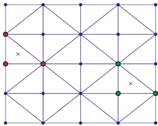
Fig. 1. T3-scheme for support nodes selection. In red are the support nodes for boundary cells and in green the ones for interior cells.
T6-scheme selects 6 nodes for a cell (Fig. 2). For an interior cell, it selects its 3 vertices plus 3
remote vertices of the three neighbouring cells. For a boundary cell, it selects the 3 vertices, 2 (or 1)
remote vertices of neighbouring cells and 1 (or 2) node nearest to the centroid of the cell. This scheme
is usually used for building PIM shape function with radial basis functions, aiming to generate
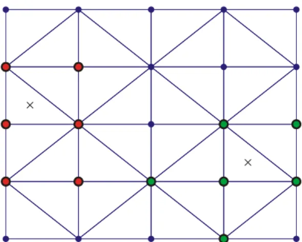
Fig. 2. T6-scheme for support nodes selection. In red are the support nodes for boundary cells and in green the ones for interior cells.
The T6/3-scheme is a combination of T6 and T3-schemes (Fig. 3). It selects 6 nodes for
interpolation of interior cells in the same way as T6-scheme, and 3 nodes for boundary cells as in
T3-scheme. T6/3-scheme is used to build high-order PIM shape functions, where linear interpolation is
performed on boundary and quadratic interpolation is performed in the interior.
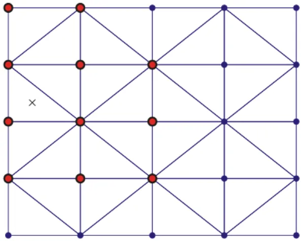
Fig. 3. T6/3-scheme for support nodes selection. In red are the support nodes for boundary cells and in green the ones for interior cells.
T2L-scheme selects two layer of nodes (Fig. 4). The first layer corresponds to the 3 vertices of the
cell and the second layer holds the nodes that are directly connected to the first layer nodes. This
scheme generally selects more nodes than T6-scheme, leading to bigger computational costs.
T2L-scheme is used to build PIM shape functions with radial basis functions with higher order of
consistency and when the nodal distribution is very irregular. T2L-scheme can also be employed to
build MLS shape functions.
D. Construction of the Smoothing Domains
As seen in Section II-C, smoothed gradients are calculated based on smoothing domains. The
procedure for construction of these domains leads to different numerical approximation
characteristics. Two requirements are imposed on the smoothing domains: (I) the intersection between
the subdomains must completely cover the problem domain. Three point interpolation methods based
on smoothing gradients derive from the way that the smoothing domains are constructed: NS-PIM,
ES-PIM and CS-PIM.
Fig. 4. T2L-scheme for support nodes selection.
The Node-Based Smoothing Point Interpolation Method (NS-PIM) [8] constructs the smoothing
domains based on the nodes of the triangular mesh. For each node , a smoothing domain is
created connecting sequentially the centroid of the cells which are incident to node to the
mid-edge-points, as it can be seen in Fig. 5. Therefore, the number of smoothing subdomains is equal to number
of nodes in the mesh, and the requirements (I) and (II) are met.
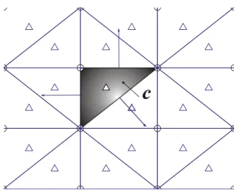
Fig. 5. Node based smoothing subdomain . The centroids of the cells are represented by triangles and mid-edge-points by diamonds. The unit outwards normals on are represented by vectors.
The Edge-Based Smoothing Point Interpolation Method (ES-PIM) [9] constructs its smoothing
domains based on the edges of the triangular mesh. For each edge , a smoothing domain is
created connecting the endpoints of edge to the centroids of the adjacent cells, as shown in Fig. 6.
Clearly, requirements (I) and (II) are met, and the number of smoothing domains corresponds to the
number of edges in the mesh.
The Cell-Based Smoothing Point Interpolation Method (CS-PIM) [10] constructs its smoothing
as shown in Fig. 7. For that reason, CS-PIM is very similar to the finite element method.
Requirements (I) and (II) are met and the number of smoothing domains matches the number of
triangles in the mesh.
Fig. 6. Edge based smoothing subdomain . The centroids of the cells are represented by triangles. The unit outwards normals on are represented by vectors.
Fig. 7. Cell based smoothing subdomain . The centroids of the cells are represented by triangles. The unit outwards normals on are represented by vectors.
IV. NUMERICAL RESULTS
In this section we investigate the performance of the gradient smoothing methods presented in
Section III. In the following problems, the errors on the approximated potentials are calculated using a
set of sampled points. The error measure is defined as
√∑ ( )
∑ ( ) (31)
where is the number of sampled points, is the analytical solution at the th point and is the
A. Example 1: Parallel Plate Capacitor
The first test problem is the parallel plate capacitor with one dielectric. The goal is to verify if the
methods can reproduce a linear field, represented by the electric potential. The plates are located at
and and are at voltages 100V and 10V, respectively. The problem analytical solution is
(32)
A distribution of 5 5 nodes is used in a square domain with the dimension of 1 1. We test the
methods NS-PIM, ES-PIM and CS-PIM with T3-scheme. The norm of error are 3.67 10-16, 2.04
10-16 and 1.86 10-16, respectively. This example shows numerically that the three methods can
reproduce linear fields exactly (to machine accuracy), which ensures a second order convergence in
norm [1].
B. Example 2: Parallel Plate Capacitor with Two Dielectric
The problem of Example 1 is revisited, but with the presence of two dielectrics having relative
permittivities of 1 and 5. The interface between the two dielectric is at . The purpose of this
example is to test whether the methods can treat discontinuities in the solution due to the presence of
different media in the domain. The problem analytical solution is
{ (33)
Again, a distribution of 5 5 nodes is used. We test NS-PIM, ES-PIM and CS-PIM with
T3-scheme. The norm of error are 1.16 10-16, 7.12 10-17 and 5.36 10-17, respectively. The results
show that the three methods can reproduce exactly (to machine accuracy) the discontinuity of the
solution at the interface between the materials.
C. Example 3: Square Domain with Senoidal Dirichlet Boundary Condition
In this example we test the methods against a problem with a senoidal Dirichlet boundary condition.
The problem domain is a square with the dimension of 1 1, as shown if Fig. 8. The boundaries at
, and are at an electric potential of 10V. The top boundary ( ) has a potential given by a sine function with a maximum value of 100V. We test NS-PIM, ES-PIM and CS-PIM with
T-schemes and shape functions generated by PIMp and RPIMp with Multiquadrics RBF [1]. The
problem analytical solution is
(34)
The first step is to verify if the models can approximate the electric potential correctly. For so, the
solution is computed along the line for the models NS-PIM with T6/3-scheme, ES-PIM with
T3 and T6/3 schemes and, finally, ES-PIM with shape functions generated by RPIMp (ES-RPIM) and
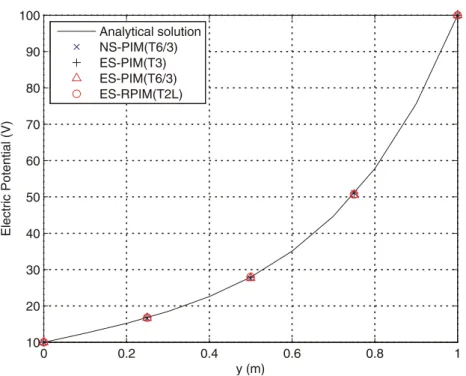
T2L-scheme for support nodes selection. Fig. 9 shows the analytical and numerical solutions for
comparison. It can be seen that the results produced by all the models are in accordance with the
Fig. 8. Problem domain of Example 3.
Fig. 9. Electric potential along calculated using different methods based on gradient smoothing.
In order to investigate the convergence rate of the methods to the exact solution, four nodes
distributions are used to calculate the error in norm of . We also test the finite element method for
comparison. All models use the same sets of nodes and the same meshes. Fig. 10 shows the solution
error on logarithm scale for different nodal densities represented by the nodal spacing . As expected,
FEM achieves a convergence rate around 2.0 (2.04), which is the theoretical value for linear models
based on weak forms. CS-PIM produces the same numerical solution than FEM, which is also
expected because its smoothing domains are the triangles of the mesh. Except the quadratic ES-PIM,
that has a rate of 1.94, all the methods have convergence rates greater than the finite element method.
It can be observed that the node based smoothing methods are less accurate than FEM. On the other
hand, the edge based smoothing methods generate the best results, especially when they build their
which select more support nodes for building the shape functions and increase the accuracy of the
approximation.
The highest convergence rate (2.36) is obtained by ES-RPIM with T2L-scheme, indicating the
presence of superconvergence [1]. Another model with a good rate (2.24) is the ES-PIM with
T3-scheme, whose solution is also more accurate than FEM. This method is particularly interesting
because it uses few support nodes, having thus a good computational efficiency in terms of memory
usage and run time, and also it has no parameter to be adjusted as the models that use RBFs.
According to the authors' experience, determining these parameters is a hard task because they can
vary from problem to problem, meaning that there is not a deterministic way for calculating them,
while their values impact significantly on the quality of the numerical solution.
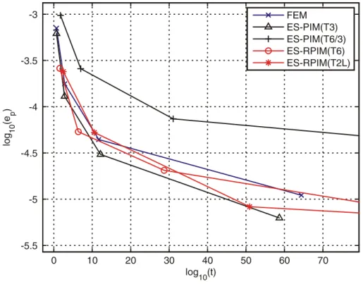
Fig. 10. Convergence rates in norm of error for gradient smoothing methods and FEM.
Proceeding with the investigation of the characteristics of the smoothing methods, an analysis
relative to the computational efficiency of the models is performed. Since the edge based smoothing
models presented the best results for convergence rate and accuracy, they are the only ones that are
put to the test.
It is known that the finite element method has a computational processing time considerably lower
than the traditional meshless methods, namely EFG and MLPG, when considering that they use the
same set of nodes. However, a fairer comparison is to evaluate the computational performance with
respect to the accuracy of the numerical approximation. Following this line, the finite element method
against the gradient smoothing methods. The errors in norm of as a function of processing time
spent by the models are shown in Fig. 11. All the smoothing models, except ES-PIM (T6/3), have
computational efficiency comparable to the finite element method. In particular, it can be seen that
ES-PIM with T3-scheme is the most computational efficient in terms of run time, as previously
pointed out, and it overcomes even the finite element method for the considered scenario. This result
is due to the fact that ES-PIM (T3) generates more accurate solution than FEM for the same mesh
with a not so much more processing time, that is, the difference between the processing time are
compensated with a greater accuracy for the gradient smoothing method.
Fig. 11. Computational efficiency comparison for gradient smoothing methods and FEM. Error in norm of vs processing time.
D. Example 4: Radial Magnetic Bearing
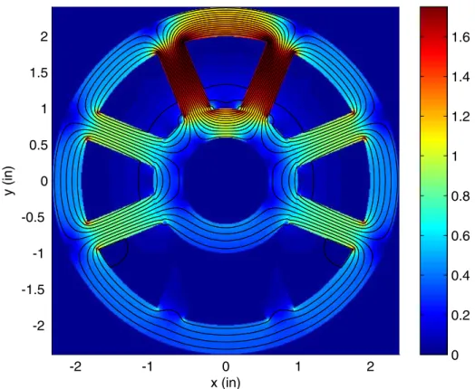
This example deals with an eight pole radial magnetic bearing taken from [11]. Fig. 12 shows the
bearing geometry. In the original example, the ferromagnetic material has a nonlinear - curve. In
this work, the nonlinearity is neglected for simplicity.
The example is a magnetostatic problem where the unknown is the magnetic vector potential in
-direction. The magnetic flux density is computed in the entire bearing using ES-PIM with
T3-scheme and a mesh of 20513 nodes and 40464 triangular elements (Fig. 13). The flux lines are
Fig. 12. Eight pole radial magnetic bearing. Dimensions are in inches. Figure taken from [11].
Fig. 13. Magnetic flux density (T) computed by ES-PIM with T3-scheme. Flux lines are also shown.
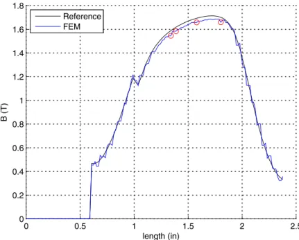
The previous mesh is used by ES-PIM and FEM to compute at a radial segment in the upper left
approximation generated by FEM using a mesh with 189492 nodes and 377677 triangular elements.
The results are shown in Fig. 14 and 15 for ES-PIM and FEM, respectively. It can be seen that at the
central region of the leg, ES-PIM is more accurate than FEM. The four maximum absolute percentual
errors for each model are computed and indicated with red circles in the figures, and their values are
listed in Table I.
Fig. 14. Magnetic flux density (T) computed by ES-PIM with T3-scheme at a radial segment in the upper left leg. Red circles indicate where the four max percentual differences occur in the center region of the leg.
TABLE I.MAXIMUM ABSOLUTE PERCENTUAL ERROR (%) FOR MAGNETIC DENSITY FLUX IN THE CENTRAL REGION OF THE UPPER LEFT LEG OF THE BEARING OF ES-PIM AND FEM NUMERICAL SOLUTIONS.
ES-PIM (T3) FEM
1.77 2.71 1.66 2.44 1.21 2.12 1.20 2.07
V. CONCLUSION
An study of meshless point interpolation methods based on weakened-weak forms with gradient
smoothing was presented. The methods NS-PIM, ES-PIM and CS-PIM and their formulations for
static problems were derived. Four numerical examples were solved, covering both electrostatics and
magnetostatics.
The numerical results showed that the gradient smoothing methods have convergence rates of the
same order or higher than the finite element method, as suggested for models with W2 formulations.
Edge based smoothing methods have the best convergence rates and accuracies. In addition, these
models presented comparable or higher computational efficiency than the finite element method when
accuracy is considered.
An eight pole radial magnetic bearing problem was solved to test ES-PIM in a real and more
complex problem. It was shown that the approximation generated by ES-PIM is also better than the
one generated by FEM for this problem.
In general, edge based smoothing models proved to be the most attractive in terms of convergence
rate, accuracy and computational efficiency. In particular, ES-PIM with T3-scheme is chosen by the
author as the best gradient smoothing model.
ACKNOWLEDGMENT
This work was supported in part by the State of Minas Gerais Research Foundation - FAPEMIG,
Brazil, the Brazilian government agency CAPES and National Council for Scientific and
Technological Development - CNPq, Brazil.
REFERENCES
[1] G. R. Liu, Mesh Free Methods: Moving Beyond the Finite Element Method, 2nd ed. CRC Press, 2009.
[2] T. Belytschko, Y. Y. Lu, and L. Gu, “Element-free Galerkin methods,” International Journal for Numerical Methods in Engineering, vol. 37, no. 2, pp. 229 – 256, 1994.
[3] S. N. Atluri and S. Shen, “The meshless local Petrov-Galerkin (MLPG) method - A simple and less-costly alternative to
the finite element and boundary element methods,” CMES - Computer Modeling in Engineering and Sciences, vol. 3, no. 1, pp. 11–51, 2002.
[4] N. Z. Lima, R. C. Mesquita, W. G. Facco, A. S. Moura, and E. J. Silva, “The nonconforming point interpolation method
applied to electromagnetic problems,” IEEE Transactions on Magnetics, vol. 48, pp. 619–622, 2012.
[5] G. Liu, “A g space theory and a weakened weak (w2) form for a unified formulation of compatible and incompatible methods: Part i theory and part ii applications to solid mechanics problems,” International Journal for Numerical Methods in Engineering, vol. 81, pp. 1093–1126, 2010.
[6] T. J. R. Hughes, The Finite Element Method: Linear Static and Dynamic Finite Element Analysis. Dover Publications, 2000.
[8] S. Wu, G. Liu, H. Zhang, and G. Zhang, “A node-based smoothed point interpolation method (ns-pim) for thermoelastic
problems with solution bounds,” International Journal of Heat and Mass Transfer, vol. 52, pp. 1464–1471, 2009. [9] S. Wu, G. Liu, X. Cui, T. Nguyen, and G. Zhang, “An edge-based smoothed point interpolation method (es-pim) for
heat transfer analysis of rapid manufacturing system,” International Journal of Heat and Mass Transfer, vol. 53, pp.
1938–1950, 2010.
[10]G. Zhang and G.-R. Liu, “A meshfree cell-based smoothed point interpolation method for solid mechanics problems,” AIP Conference Proceedings, vol. 1233, no. 1, pp. 887–892, 2010.