Int. J. Adv. Appl. Math. and Mech. 2(3) (2015) 38 - 50 (ISSN: 2347-2529) Journal homepage:www.ijaamm.com
International Journal of Advances in Applied Mathematics and Mechanics
Application of meshless local radial point interpolation
(MLRPI) on generalized one-dimensional linear telegraph
equation
Research Article
Elyas Shivanian
∗, Hamid Reza Khodabandehlo
Department of Mathematics, Imam Khomeini International University, Qazvin, 34149-16818, Iran
Received 02 December 2014; accepted (in revised version) 28 February 2015
Abstract:
In this paper, the meshless local radial point interpolation (MLRPI) method is applied to generalized one-dimensional linear telegraph equations. The MLRPI method is one of the â ˘AIJtruly meshlessâ ˘A˙I methods since it does not require any background integration cells so that all integrations are carried out locally over small quadrature domains of regular shapes, such as lines in one dimensions, circles or squares in two dimensions and spheres or cubes in three dimensions. A technique is proposed to construct shape functions using radial ba-sis functions. These shape functions, which are constructed by point interpolation method using the radial baba-sis functions, have delta function property. The time derivatives are approximated by the time-stepping method. Numerical experiments of this method are carried out and compared with Fourth-order compact difference and alternating direction implicit method.MSC:
65N12• 65N1•65N30Keywords:
Local weak formulation• Meshless local radial point interpolation• (MLRPI) method; Radial basis function•Telegraph equations c
2015 IJAAMM all rights reserved.
1.
Introduction
The telegraph equation is one of the important equations of mathematical physics with applications in many dif-ferent fields such as transmission and propagation of electrical signals[1,2], vibrational systems[3], random walk theory[4], and mechanical systems[5], etc. The heat diffusion and wave propagation equations are particular cases of the telegraph equation. Recently, increasing attention has been paid to the development, analysis, and imple-mentation of stable methods for the numerical solutions of second-order hyperbolic equations. There have been many numerical methods for hyperbolic equations, such as the finite difference, the finite element, and the colloca-tion methods, etc. see[6–21]and literatures are therein. Mohanty et al.[17,18]developed some alternating direction implicit schemes for the two and three-dimensional linear hyperbolic equations. Most of these schemes are second-order accurate in both space and time. Some conditionally stable fourth-second-order compact difference schemes for the wave and telegraph equations were introduced in[8,9,13]. An advantage of compact difference schemes is that the schemes use narrower stencils, i.e., fewer neighboring nodes, and have less truncation error comparing to typical finite difference schemes. Various versions of compact schemes have been successfully developed and analyzed [22,23]. The alternating direction implicit (ADI) methods were first introduced by Douglas, Peaceman, and
Rach-ford[24–27], which have an advantage of no increase in dimension of the coefficient matrices corresponding matrix
equations. There are many extensions and a great variety of applications of ADI based on the finite difference or the finite element methods[28–33]. In[36], Xie et. al. have proposed two and three-level compact difference and
∗ Corresponding author.
ADI compact difference schemes with high accuracy for numerical solutions of the one and two-dimensional tele-graph equations with Dirichlet boundary conditions. These compact schemes are unconditionally stable and have a truncation error of second and fourth-order in time and space, respectively. The coefficient matrices of the matrix equations given by the schemes are symmetric and tridiagonal. The matrix equations can be effectively solved by using many linear solvers. Numerical experiments presented for the 1D and 2D telegraph equations show that the present schemes are of high accuracy. By comparing the numerical results obtained by the present methods with the ones of some other available methods, the present methods can be considered as practical and effective numerical techniques to solve telegraph equations. LetΩ= (0,X). Consider the 1D linear telegraph equation
∂2u
∂t2 +c ∂u
∂t +b u −p
∂2u
∂x2 = f(x,t), (x,t)∈Ω×(0,T], (1) with the initial and boundary conditions
u(x, 0) =u0(x), ∂u
∂t(x, 0) =ψ(x), u(0,t) =gl(t), u(1,t) =gr(t),
(2)
wherec, b andp are positive constants and, the functionsf andψare assumed to be sufficiently smooth. The main shortcoming of mesh-based methods such as the finite element method (FEM), the finite volume method (FVM) and the boundary element method (BEM) is that these numerical methods rely on meshes or elements. In the last two decades, in order to overcome the mentioned difficulties some techniques the so-called meshless meth-ods have been proposed[37]. This method is used to establish system of algebraic equations for the whole domain of the problem without the use of predefined mesh for the domain discretization so that set of nodes scattered within the domain of the problem as well as sets of nodes on the boundaries of the domain to represent (but not to discretize) the domain of the problem and its boundaries is used. These sets of scattered nodes are usually called field nodes. There are three types of meshless methods: meshless methods basedon weakforms such as the ele-ment free Galerkin (EFG) method[38,39], meshless methods based on collocation techniques (strong forms) such as the meshless collocation method based on radial basis functions (RBFs)[40–42]and meshless methods based on the combination of weak forms and collocation technique. Due to the ill-conditioning of the resultant linear systems in RBF-collocation method, various approaches are proposed to circumvent this problem, Refs. [43–46] being among them. The weak forms are used to derive a set of algebraic equations through a numerical integration process using a set of quadrature domain that may be constructed globally or locally in the domain of the problem. In the global weak form methods, global background cells are needed for numerical integration in computing the algebraic equations. To avoid the use of global background cells, a so-called local weak form is used to develop the meshless local Petrov-Galerkin (MLPG) method[47–52,54]. When a local weak form is used for a field node, the numerical integrations are carried out over a local quadrature domain defined for the node, which can also be the local domain where the test (weight) function is defined. The local domain usually has a regular and simple shape for an internal node (such as sphere, rectangular, etc.), and the integration is done numerically within the local domain. Hence the domain and boundary integrals in the weak form methods can easily be evaluated over the regularly shaped sub-domains(spheres in 3D or circles in 2D) and their boundaries. In the literature, several meshless weak form methods have been reported such as diffuse element method (DEM)[59], smooth particle hy-drodynamic (SPH)[60,61], the reproducing kernel particle method (RKPM)[62], boundary node method (BNM)
[63], partition of unity finite element method (PUFEM)[64], finite sphere method (FSM)[65]and boundary radial
point interpolation method (BRPIM)[66]. Liu applied the concept of MLPG and developed meshless local radial point interpolation (MLRPI) method[55–58,67–69]. In this paper, we concentrate on the numerical solution of the Eqs. (1) -(2) using the meshless local radial point interpolation (MLRPI) method. Some examples are given to com-pare the results with those obtained by Fourth-order compact difference and alternating direction implicit method to show the high accuracy of the present method.
2.
The modified radial point interpolation scheme
In the conventional point interpolation method (PIM) there is a main difficulty that inverse of the polynomial mo-ment matrix (it will be defined later) does not often exist. This condition could always be possible depending on the locations of the nodes in the support domain and the terms of monomials used in the basis. If an inappropriate polynomial basis is chosen for a given set of nodes, it may yield in a badly conditioned or even singular moment matrix[37]. In order to avoid the singularity problem in the polynomial point interpolation method (PIM), the radial basis function (RBF)is used to develop the radial point interpolation method (RPIM) for meshless weak form tech-niques[68,70,71]. The combination of RPIM and polynomial PIM is described as follows: consider a continuous functionu(x)defined in a domainΩ, which is represented by a set of field nodes. Theu(x)at apoint of interestxis approximated in the form of
u(x) = n X
i=1
Ri(x)ai + m X
j=1
pj(x)bj =RT(x)a+PT(x)b, (3)
WhereRi(x)is a radial basis function (RBF),nis the number of RBFs,pj(x)is monomial in the space coordinatexand
mis the number of polynomial basis functions. Thepj(x)in Eq.(3) is, in general, chosen in a top-down approach
from the Pascal triangle, so that the basis is complete to a desired order and a complete basis is usually preferred. For 1D problems, We use
PT(x) =1,x,x2,x3, ...,xm , (4)
For 2D problems, We sall have
PT(x) =PT(x,y) =1,x,y,x y,x2,y2, ...,xm,ym , (5)
And etc. Whenm =0, onlyRBFsareused. Otherwise, the RBF is augmented withm polynomial basis functions. Coefficientsai andbj are unknown which should be determined. There are a number of types of RBFs, and the
characteristics of RBFs have been widely investigated[40,72,73]. In the current work, we have chosen the thin plate spline (TPS) as radial basis functions in Eq.(3). This RBF is defined as follows:
R(x) =r2m ln(r), m =1 , 2 , 3 , ... . (6)
SinceR(x)in Eq.(6) belongs toC2m−1(all continuous function to the order2m−1), so higher-order thin plate splines must be used for higher-order partial differential operators. For the second-order partial differential equation (1), m =2 is used for thin plate splines (i.e., second-order thin plate splines). In the radial basis functionRi(x), the
variable is only the distance between the point of interestx and a node atxi, i.e.,r =|x − xi |for 1-D andr = p
(x −xi)2+ (y −yi)2 for 2-D. In order to determineai andbjin Eq.(3), a support domain is formed for the point
of interest at x, andn field nodes are included in the support domain. Coefficientsai and bj in Eq.(3) can be
determined by enforcing Eq.(3) to be satisfied at thesennodes surrounding the point of interestx. This leads to the system ofnlinear equations, one for each node. The matrix form of these equations can be expressed as
Us =Rna+Pmb. (7)
where the vector of function valuesUsis
Us ={u1,u2,u3, ... ,un}T , (8)
the RBFs moment matrix is
Rn =
R1(r1) R2(r1) ... Rn(r1)
R1(r2) R2(r2) ... Rn(r2) ..
. ... ... ... R1(rn) R2(rn) ... Rn(rn)
n×n
, (9)
and the polynomial moment matrix is
Pm =
1 x1 ... x1m 1 x2 ... x2m
..
. ... ... ... 1 xn ... xnm
n×m
. (10)
Also, the vector of unknown coefficients for RBFs is
aT ={a1,a2,a3, ... ,an}, (11)
and the vector of unknown coefficients for polynomial is
bT ={b1,b2,b3, ... ,bm}, (12)
We notify that, in Eq.(9),rk inRi(rk)is defined as
rk =|xk −xi | . (13)
We mention that there arem +nvariables in Eq.(7). The additionalmequations can be added using the following mconstraint conditions:
n X
i=1
Combining Eqs.(7) and (14) yields the following system of equations in the matrix form:
˜ Us =
Us
0
=
Rn Pm
PT
m 0
a b
=Ga˜, (15)
where
˜
Us ={u1u2...un0 0 ... 0}, a˜T ={a1a2...anb1...bm}. (16)
Because the matrixRnis symmetric, the matrixG will also be symmetric. Solving Eq.(15), we obtain
˜ a=
a b
=G−1U˜s. (17)
Eq.(3) can be rewritten as
u(x) =RT(x)a+PT(x)b =RT(x),PT(x)
a b
. (18)
Now using Eq.(17), we obtain
u(x) =RT(x),PT(x) G−1U˜s =Φ˜T(x)U˜s, (19)
where ˜ΦT(x)can be rewritten as
˜
ΦT(x) =RT(x),PT(x) G−1 =φ1(x)φ2(x)...φn(x)φn+1(x)...φn+m(x) . (20)
The firstnfunctions of the above vector function are called the RPIM shape functions corresponding to the nodal displacements. We show by the vector ˜ΦT(x)so that it is
˜
ΦT(x) =φ1(x)φ2(x)...φn(x) . (21)
then Eq.(19) is converted to the following one:
u(x) =Φ˜T(x)Us = n X
i=1
φi(x)ui. (22)
The derivatives ofu(x)are easily obtained as
∂u(x)
∂x =
n X
i=1 ∂ φi(x)
∂x ui,
∂2u(x) ∂x2 =
n X
i=1 ∂2φ
i(x)
∂x2 ui. (23)
Note thatR−n1usually exists for arbitrary scattered nodes and therefore the augmented matrixGis theoretically non-singular[74,75]. In addition, the order of polynomial used in Eq.(3) is relatively low. We add that the RPIM shape functions have the Kronecker delta function property, that is
φi(xj) = §1 ,
i = j, j =1 , 2, ... ,n,
0 , i 6= j, j =1 , 2, ... ,n. (24)
This is be cause the RPIM shape functions are created to pass through nodal values.
3.
The time discretization approximation
In the current work, We employ a time-stepping scheme to approximate the time derivative. For this purpose, the following finite difference approximation can be used:
∂2u(x,t)
∂t2 ∼= 1
∆t2 u
k+1(x)−2uk(x) +uk−1(x)
, (25)
∂u(x,t)
∂t ∼
= 1
2∆t u
k+1(x)−uk−1(x)
, (26)
Also we employ the following approximation by using the Crank-Nicolson technique:
u(x,t)∼= 1
3 u
k+1(x) +uk(x) +uk−1(x)
, ∂2u(x,t)
∂x2 ∼= 1 3
∂2uk+1(x,t) ∂x2 +
∂2uk(x,t)
∂x2 +
∂2uk−1(x,t) ∂x2
, (27)
whereuk(x) =u(x,k∆t).
Using the above discussion, Eq.1can be written as:
1
∆t2 u
(k+1)(x)−2u(k)(x) +u(k−1)(x)
+ c
2∆t u
(k+1)(x)−u(k−1)(x)
+b
3 u
(k+1)(x) +u(k)(x) +u(k−1)(x)
− p 3
∂2u(k+1)(x)
∂x2 +
∂2u(k)(x)
∂x2 +
∂2u(k−1)(x)
∂x2
= 1
3 f
(k+1)(x) + f(k)(x) +f(k−1)(x)
,
(28)
Suppose thatλ= 1
∆t2,µ= c
2∆t, then we obtain
λ u(k+1)(x)−2u(k)(x) +u(k−1)(x)
+µ u(k+1)(x)−u(k−1)(x)
+b
3 u
(k+1)(x) +u(k)(x) +u(k−1)(x)
− p 3
∂2u(k+1)(x)
∂x2 +
∂2u(k)(x)
∂x2 +
∂2u(k−1)(x)
∂x2
= 1
3 f
(k+1)(x) + f(k)(x) +f(k−1)(x)
,
(29)
thus
λ+µ+ b
3
u(k+1)−p 3
∂2u(k+1)(x)
∂x2 =
2λ− b 3
u(k)+p
3
∂2u(k)(x)
∂x2
+
−λ+µ− b 3
u(k−1)+p 3
∂2u(k−1)(x)
∂x2 + 1 3 f
(k+1)(x) + f(k)(x) + f(k−1)(x)
.
(30)
4.
The meshless local weak form formulation
Instead of giving the global weak form, the MLRPI method constructs the weak form over local quadrature cell such asΩq, which is a small region taken for each node in the global domainΩ. The local quadrature cells
over-lap with each other and cover the whole global domain Ω. The local quadrature cells could be of any geomet-ric shape and size. In one dimensional problems, they are line (interval). The local weak form of Eq.(30) for xi ∈Ωiq = xi −rq,xi +rq
. can be written as
R Ωi
q(
λ+µ+ b
3
u(k+1)−p 3
∂2u(k+1)( x)
∂x2 )ν(x)d x=
R Ωi
q(
2λ− b 3
u(k)
+p
3
∂2u(k)(x)
∂x2 )ν(x)d x+
R
Ωi q(
−λ+µ− b 3
u(k−1)+p 3
∂2u(k−1)(x)
∂x2 )ν(x)d x
+R
Ωi q(
1 3 f
(k+1)(
x) + f(k)(
x) + f(k−1)(
x))ν(x)d x,
(31)
whereΩi
qis the local quadrature domain associated with the pointi, andν(x)is the Heaviside step function[76,77]:
ν(x) = §1 ,
x ∈Ωq,
0 , x ∈/Ωq, (32)
as the test function in each local quadrature domain. Hence, we have
λ+µ+ b
3
R
Ωi q u
(k+1)ν(x)d x −p 3
R
Ωi q
∂2u(k+1)(x)
∂x2 ν(x)d x
=
2λ− b 3
R
Ωi q u
(k)ν(x)d x +p 3
R
Ωi q
∂2u(k)(x)
∂x2 ν(x)d x
+
−λ+µ− b 3
R
Ωi q u
(k−1)ν(x)d x +p 3
R Ωi
q
∂2u(k−1)( x)
∂x2 ν(x)d x
+1
3
R
Ωi q f
(k+1)(x) + f(k)(x) + f(k−1)(x)
ν(x)d x,
(33)
Using integration by parts, one has:
Z
Ωi q
∂2u(k)(x)
∂x2 ν(x)d x =ν(x)
∂u(k)(x)
∂x | x=xi+rq x=xi−rq −
Z
Ωi q
∂u(k)(x)
∂x
∂ ν(x)
and using the test function the following local weak equation will be obtained:
λ+µ+ b
3
R
Ωi q u
(k+1)d x −p 3
∂u(k+1)(x)
∂x | x=xi+rq x=xi−rq
=
2λ− b 3
R
Ωi q u
(k)d x + p 3
∂u(k)(x)
∂x | x=xi+rq x=xi−rq
+
−λ+µ− b 3
R
Ωi q u
(k−1)d x +p 3
∂u(k−1)(x)
∂x | x=xi+rq x=xi−rq
+1 3 R Ωi q f
(k+1)(x) + f(k)(x) + f(k−1)(x)
d x.
(35)
Applying the radial point interpolation method (RPIM) for the unknown functions, the local integral equation (35) is transformed in to a system of algebraic equations with used unknown quantities, as described in the next section.
5.
Discretization for MLRPI method
In this section, we consider Eq.(35) to see how to obtain discrete equations. ConsiderNregularly located points on the boundary and domain of the problem so that the distance between two consecutive nodes in each direction is constant and equal toh. Assuming thatu(xi,k∆t),i=1, 2, ...,Nare known,our aim is to computeu(xi,(k+1)∆t),i=
1, 2, ...,N. So, we haveNunknowns and to compute these unknowns we needNequations. As it will be described, corresponding to each node we obtain one equation. For nodes which are located in the interior of the domain, i.e., forxi ∈interiorΩ, to obtain the discrete equations from the locally weak forms (35), substituting approximation
formulas (22) and (23) in to local integral equations (35) yields
λ+µ+b
3
PN
j=1
R
Ωi
qφj(x)d x
u(jk+1)−p 3
PN
j=1
∂ φj(x)
∂x |x=xi+rq−
∂ φj(x)
∂x |x=xi−rq
u(jk+1)
=
2λ−b 3
PN
j=1
R
Ωiqφj(x)d x
u(jk)+p
3
PN
j=1
∂ φj(x)
∂x |x=xi+rq−
∂ φj(x)
∂x |x=xi−rq
u(jk)
+
−λ+µ−b 3
PN
j=1
R
Ωi qφj
(x)d x
u(jk−1)+p
3
PN
j=1
∂ φj(x)
∂x |x=xi+rq−
∂ φj(x)
∂x |x=xi−rq
u(jk−1)
+1
3
R
Ωi q f
(k+1)(x) + f(k)(x) +f(k−1)(x)
d x.
(36)
or equivalently
λ+µ+b
3
PN
j=1
R
Ωi qφj
(x)d x
−p 3
PN
j=1
∂ φj(x)
∂x |x=xi+rq−
∂ φj(x)
∂x |x=xi−rq
u(jk+1)
=
2λ−b 3
PN
j=1
R
Ωi
qφj(x)d x
+p
3
PN
j=1
∂ φj(x)
∂x |x=xi+rq−
∂ φj(x)
∂x |x=xi−rq
u(jk)
+
−λ+µ−b 3
PN
j=1
R
Ωiqφj(x)d x
+p
3
PN
j=1
∂ φj(x)
∂x |x=xi+rq−
∂ φj(x)
∂x |x=xi−rq
u(jk−1)
+1
3
R
Ωi q f
(k+1)(
x) + f(k)(
x) +f(k−1)( x)d x.
(37)
6.
Numerical implementation for MLRPI method
For nodes which are located on the boundary, we have
∀k :uk(xi) =0 , xi ∈∂Ω={0 ,X}. (38)
The matrix forms of Eqs.(37) and (38) for allN nodal points in domain and in boundary of the problem are given below:
λ+µ+ b
3
PN
j=1Ai,j −
p 3
PN
j=1Bi,j
u(jk+1)
=
2λ− b 3
PN
j=1Ai,j +
p 3
PN
j=1Bi,j
u(jk)
+
−λ+µ− b 3
PN
j=1Ai,j +
p 3
PN
j=1Bi,j
u(jk−1)+Ei(k−1,k,k+1),
(39)
where Ai,j =
R Ωi
q φj(x)d x, Bi,j =
∂ φj(x)
∂x |x=xi+rq −
∂ φj(x)
∂x |x=xi−rq
,
Ei(k−1,k,k+1) =
1 3
R Ωi
q f
(k+1)(x) + f(k)(x) + f(k−1)(x)
d x.
(40)
AssumingAi,j =
λ+µ+b
3
Ai,j−
p
3 Bi,j,Bi,j =
2λ−b 3
Ai,j+
p
3Bi,j,Ci,j =
−λ+µ−b 3
Ai,j+
p
3Bi,j andE
k =
[E1(k−1,k,k+1),E2(k−1,k,k+1), ...,EN(k−1,k,k+1)]T,U= (ui)N×1. (39) yeilds
AU(k+1)=BU(k)+CU(k−1)+Ek. (41)
Furthermore, to satisfy Eq.(38), for all nodes belong to the boundary, i.e.,xi ∈∂Ω, We set
Ci,i =Eki =0 , ∀j :Bi,j =0 , Ai,j = §1 ,
i = j,
0 , i 6= j. (42)
At the first time level, whenn=0, according to the initial conditions that were introduced in Eq.(2), We apply the following assumptions:
u(0) =u0,
and
u(−1) ∼=u(1)−2ψ.
whereu0 = [u0(x1),u0(x2), ... ,u0(xN) ]T andψ= [ψ(x1), ,ψ(x2), , ... ,ψ(xN) ]T.
7.
Numerical experiments
In this section the numerical results obtained from application of the meshless local radial point interpolation method (MLRPI) for solving the one-dimensional linear telegraph equation are presented. We show the results obtained for two examples using the meshless method described above. In both examples, the domain integrals are evaluated with 7 points Gaussian quadrature rule. These examples are chosen for comparison with the results of Fourth-order compact difference and alternating direction implicit schemes[36]. In all problems, the regular node distribution is used. Also in order to implement the meshless local weak form in all cases considered, the radius of the local quadrature domainrq = 0.8his selected, wherehis the distance between the nodes inx direction
(h =∆x). The size ofrq is such that the union of these sub-domains must cover the whole global domain. The
radius of support domain to local radial point interpolation method isrs=4rq . This size is significant enough to
have sufficient number of nodes (n) and gives an appropriate approximation. Also, in Eq.(3), we setm =5. Example 1. We setc = 20 ,b = 25 andp = 1. The exact solution of the first example is taken asu(x,t) =
t3x2(1−x)2,(x,t)∈[0, 1]×[0, 1]. The functionf and the initial and boundary conditions can be obtained by using the exact solution, wheref(x,t)is defined accordingly, i.e.
f(x,t) = (6t+3c t2)(x2(1−x)2) +b t3(x2(1−x)2)−p t3(12x2−12x +2),
initial condition is obviously
u(x, 0) =0 , ∂u
∂t (x, 0) =0 , and the Dirichlet boundary condition
u(0,t) =u(1,t) =0 , t ≥0.
Tables1and2as well as Figs. 1and2compares the results of MLRPI with those obtained by Fourth-order com-pact difference and alternating direction implicit scheme. As it is seen, MLRPI is superior to Fourth-order comcom-pact difference and ADI method.
Example 2. We set c = 20 ,b = 25 andp = 1. The exact solution of the this example is taken asu(x,t) =
exp(t)x2(1 −x)2,(x,t)∈[0, 1]×[0, 1]. The functionf and the initial and boundary conditions can be obtained by using the exact solution, wheref(x,t)is
f(x,t) = (e x p(t) +c e x p(t))(x2(1−x)2) +b e x p(t) (x2(1−x)2)−p e x p(t) (12x2−12x +2),
initial condition
u(x, 0) = x2(1−x)2, ∂u
∂t(x, 0) = x
2(1−x)2.
and the Dirichlet boundary condition
u(0,t) =u(1,t) =0 , t ≥0.
Table 1. TheL1,L2andL∞errors calculated by MLRPI for Example 1 with different∆xand∆t at timet =1.0.
∆t h kEk∞ kEk2 kEk1
1 10
1
10 2.934016E−004 6.075916E−004 1.632193E−003
1 20
1
20 7.186905E−005 2.151650E−004 8.312477E−004
1 40
1
40 1.781325E−005 7.591145E−005 4.212198E−004
1 80
1
80 4.438404E−006 2.678269E−005 2.109794E−004
1 160
1
160 1.107990E−006 9.458974E−006 1.054717E−004
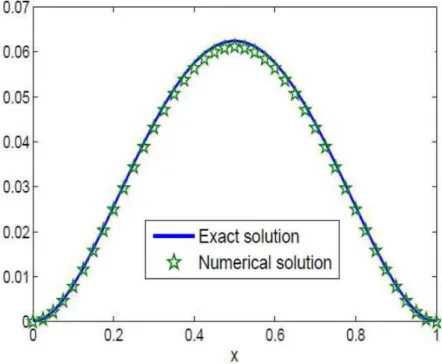
Fig. 1. Numerical solutions and exact solution at timet=1.0 for Example 1. The solid line corresponds to the exact solution, the stared line corresponds to numerical solution of the MLRPI with∆t = 401 andh= 401.
Table 2. TheL1,L2andL∞errors calculated by Fourth-order compact difference and alternating direction implicit schemes for Example 1 with different∆xand∆tat timet =1.0.
∆t h kEk∞ kEk2 kEk1
1 10
1
10 5.210669E−003 1.084486E−003 2.958748E−002
1 20
1
20 2.602278E−003 7.699436E−003 2.994501E−002
1 40
1
40 1.302337E−003 5.462982E−003 3.013781E−002
1 80
1
80 6.517098E−004 3.870778E−003 3.023497E−002
1 160
1
160 3.260200E−004 2.740052E−003 3.028345E−002
Table 3. TheL1,L2andL∞errors calculated by MLRPI for Example 2 with different∆xand∆t at timet =1.0.
∆t h kEk∞ kEk2 kEk1
1 10
1
10 3.288094E−004 5.101931E−004 1.293387E−003
1 20
1
20 4.861794E−005 1.440098E−004 5.548190E−004
1 40
1
40 1.134793E−005 4.863192E−005 2.684251E−004
1 80
1
80 2.716901E−006 1.660324E−005 1.311619E−004
1 160
1
160 6.630035E−007 5.742977E−006 6.441918E−005
Fig. 2. Numerical solutions and exact solution at timet=1.0 for Example 1. The solid line corresponds to the exact solution, the stared line corresponds to numerical solution of the Fourth-order compact difference and alternating direction implicit schemes with∆t = 401 andh= 401.
Fig. 3. Numerical solutions and exact solution at timet=1.0 for Example 2. The solid line corresponds to the exact solution, the stared line corresponds to numerical solution of the MLRPI with∆t = 401 andh= 401.
Table 4. TheL1,L2andL∞errors calculated by Fourth-order compact difference and alternating direction implicit schemes for Example 2 with different∆xand∆tat timet =1.0.
∆t h kEk∞ kEk2 kEk1
1 10
1
10 1.755578E−003 3.363310E−003 8.484398E−003
1 20
1
20 1.106923E−003 3.175334E−003 1.205161E−002
1 40
1
40 6.123678E−004 2.540998E−003 1.390194E−002
1 80
1
80 3.211329E−004 1.903373E−003 1.483812E−002
1 160
1
Fig. 4. Numerical solutions and exact solution at timet=1.0 for Example 2. The solid line corresponds to the exact solution, the stared line corresponds to numerical solution of the Fourth-order compact difference and alternating direction implicit schemes with∆t = 401 andh= 401.
8.
Conclusions
In this paper meshless local radial point interpolation (MLRPI) method has been applied to solve linear telegraph equations. The present method provides a local quadrature domain and a local support domain for each node so that the integration and the interpolation are done on these domains. In this method, the shape functions have been constructed by the radial point interpolation method. A time stepping scheme was employed to approximate the time derivative. The Heaviside step function was used as the test function in the local weak form method in MLRPI. All integrations are regular, therefore the Gaussian quadrature rule was used to calculate the numerical integration for local weak form. In the current work, to demonstrate the accuracy and usefulness of this method, two numerical examples have been presented. As demonstrated by the computational results, it is very easy to implement the proposed method for similar problems.
Acknowledgements
The authors would like to thank the referees for their valuable comments and suggestions to improve the quality of the paper.
References
[1] E. A. Gonzalez-Velasco, Fourier Analysis and Boundary Value Problems, Academic Press, New York, 1995. [2] P. M. Jordan, A. Puri, Digital signal propagation in dispersive media, J. Appl. Phys. 85 (3) (1999) 1273-1282. [3] W. E. Boyce, R. C. DiPrima, Differential Equations Elementary and Boundary Value Problems, Wiley, New York,
1977.
[4] J. Banasiak, J. R. Mika, Singularly perturbed telegraph equations with applications in the random walk theory, J. Appl. Math. Stoch. Anal. 11 (1) (1998) 9-28.
[5] A. N. Tikhonov, A. A. Samarskii, Equations of Mathematical Physics, Dover, New York, 1990.
[6] P. Almenar, L. Jodar, J. A. Martin, Mixed problems for the time-dependent telegraph equation: Continuous nu-merical solutions with a priori error bounds, Math. Comput. Modelling 25 (11) (1997) 31-44.
[7] R. Aloy, M. C. Casabà ˛an, L. A. Caudillo-Mata, L. Jøsdar, Computing the variable coefficient telegraph equation using a discrete eigenfunction method, Comput. Math. Appl. 54 (2007) 448-458.
[8] M. Ciment, S. H. Leventhal, Higher order compact implicit schemes for the wave equation, Math. Comp. 29 (1975) 985-994.
[9] M. Ciment, S. H. Leventhal, A note on the operator compact implicit method for the wave equation, Math. Comp. 32 (1978) 143-147.
[10] G. Dahlquist, On accuracy and unconditional stability of linear multi-step methods for second order differential equations, BIT 18 (1978) 133-136.
[11] M. Dehghan, A. Mohebbi, High order implicit collocation method for the solution of two-dimensional linear hyperbolic equation, Numer. Methods PDEs 25 (2009) 232-243.
[12] M. Dehghan, A. Shokri, A numerical method for solving the hyperbolic telegraph equation, Numer. Methods PDEs 24 (2008) 1080-1093.
[13] H. Ding, Y. Zhang, A new fourth-order compact finite difference scheme for the two-dimensional second-order hyperbolic equation, J. Comp. Appl. Math. 230 (2009) 626-632.
[14] M. S. El-Azab, M. El-Gamel, A numerical algorithm for the solution of telegraph equations, Appl. Math. Comput. 190 (2007) 757-764.
[15] L. Jódar, D. Goberna, Analytic-numerical solution with a priori error bounds for coupled time-dependent tele-graph equations: Mixed problems, Math Comput. Modelling 30 (1999) 39-53.
[16] R. K. Mohanty, An unconditionally stable difference scheme for the one-space dimensional linear hyperbolic equation, Appl. Math. Lett. 17 (2004) 101-105.
[17] R. K. Mohanty, M. K. Jain, An unconditionally stable alternating direction implicit scheme for the two space dimensional linear hyperbolic equation, Numer. Methods PDEs 17 (2001) 684-688.
[18] R. K. Mohanty, M. K. Jain, U. Arora, An unconditionally stable ADI method for the linear hyperbolic equation in three space dimensions, Int. J. Comput. Math. 79 (2002) 133-142.
[19] R. K. Mohanty, M. K. Jain, K. George, High order difference schemes for the system of two space second order nonlinear hyperbolic equations with variable coefficients, J. Comp. Appl. Math. 70 (1996) 231-243.
[20] R. K. Mohanty, M. K. Jain, K. George, On the use of high order difference methods for the system of one space second order non-linear hyperbolic equations with variable coefficients, J. Comp. Appl. Math. 72 (1996) 421-431.
[21] E. H. Twizell, An explicit difference method for the wave equation with extended stability range, BIT 19 (1979) 378-383.
[22] J. Zhao, W. Dai, T. Niu, Fourth-order compact schemes of a heat conduction problem with Neumann boundary conditions, Numer. Methods PDEs 23 (2007) 949-959.
[23] J. Zhao, W. Dai, S. Zhang, Fourth-order compact schemes for solving multidimensional heat problems with Neumann boundary conditions, Numer. Methods PDEs 24 (2008) 165-178.
[24] J. Jr. Douglas, On the numerical integration of∂ 2u
∂x2+ ∂2u
∂y2 = ∂u
∂t by implicit methods, J. Soc. Indust. Appl. Math. 3 (1955) 42-65.
[25] J. Jr. Douglas, D. Peaceman, Numerical solution of two-dimensional heat flow problems, AIChE Journal 1 (1955) 505-512.
[26] J. Jr. Douglas, H. Rachford, On the numerical solution of heat conduction problems in two and three space variables, Trans. Amer. Math. Soc. 82 (1960) 421-439.
[27] D. Peaceman, H. Rachford, The numerical solution of parabolic and elliptic equations, J. Soc. Indust. Appl. Math. 3 (1955) 28-41.
[28] C. Clavero, J. L. Gracia, J. C. Jorge, A uniformly convergent alternating direction HODIE finite difference scheme for 2D time-dependent convection-diffusion problems, IMA J. Numer. Anal. 26 (2006) 155-172.
[29] C. Clavero, J. C. Jorge, F. Lisbona, G.I. Shishkin, A fractional step method on a special mesh for the resolution of multidimensional evolutionary convectionâ ˘A¸S diffusion problems, Appl. Numer. Math. 27 (1998) 211-231. [30] C. Clavero, J. C. Jorge, F. Lisbona, G.I. Shishkin, An alternating direction scheme on a nonuniform mesh for
reactionâ ˘A¸Sdiffusion parabolic problems, IMA J. Numer. Anal. 20 (2000) 263-280.
[31] S. Kim, H. Lim, High-order schemes for acoustic waveform simulation, Appl. Numer. Math. 57 (2007) 402-414. [32] H. Lim, S. Kim, J. Jr. Douglas, Numerical method for viscous and non-viscous wave equations, Appl. Numer.
Math. 57 (2) (2007) 194-212.
[33] N. N. Yanenko, The Method of Fractional Steps, Springer-Verlag, New York, 1971.
[34] F. Mohammadi, Numerical solution of Bagley-Torvik equation using Chebyshev wavelet operational matrix of fractional derivative Int. J. of Adv. in Aply. Math. and Mech., 2(1) (2014) 83-91
[35] J. H. Salman, A. S. Joudah, On new class of analytic functions defined by using differintegral operator, Int. J. of Adv. in Aply. Math. and Mech., 1(4),(2014) 1-9.
[36] S. S. Xie, S. C. Yi, T. I. Kwon, Fourth-order compact difference and alternating direction implicit schemes for telegraph equations, Computer Physics Communications 183 (2012) 552-569.
[37] G. Liu,Y. Gu, An introduction to meshfree methods and their programing. Springer. 2005.
[38] T. Belytschko,Y.Y. Lu, L. Gu, Element-free Galerkin methods. International Journal for Numerical Methods in Engineering. 37 (1994) 229-256.
[39] T. Belytschko, Y. Y. Lu, L. Gu, Element free Galerk in methods for static and dynamic fracture. International Journal of Solids and Structures. 32 (1995) 2547-2570.
[40] E. Kansa, Multiquadrics-a scattered data approximation scheme with applications to computational fluid-dynamics. I. Surface approximations and partial derivative estimates. Computers & Mathematics with Applica-tions. 19(8-9) (1990) 127-145.
[42] M. Aslefallah, D. Rostamy, K. Hosseinkhani, Solving time-fractional differential diffusion equation by theta-method Int. J. of Adv. in Aply. Math. and Mech., 2(1) (2014) 1-8.
[43] L. Ling, R. Opfer, R. Schaback,Results on meshless collocation techniques. Engineering Analysis with Boundary Elements 30(4) (2006) 247-253.
[44] L. Ling, R. Schaback, Stable and convergent unsymmetric meshless collocation methods. SIAM Journal of Nu-merical Analysis 46(3) (2008) 1097-1115.
[45] N. Libre, A. Emdadi, E. Kansa, M. Shekarchi, M. Rahimian, A fast adaptive wavelet scheme in RBF collocation for nearly singular potential PDEs. Computer Modeling inEngineering and Sciences 38(3) (2008) 263-284. [46] N. Libre, A. Emdadi, E. Kansa, M. Shekarchi, M. Rahimian, A multi resolution prewavelet-based adaptive
re-finement scheme for RBF approximations of nearly singular problems. Engineering A nalysis with Boundary Elements 33(7) (2009) 901-914.
[47] S. Atluri, T. Zhu, A new meshless local Petrov-Galerkin (MLPG) approach in computational mechanics. Com-putational Mechanics 22 (1998) 117-127.
[48] S. Atluri, T. Zhu, A new meshless local Petrov-Galerkin (MLPG) approach to nonlinear problems in computer modeling and simulation. Computer Modeling & Simulation in Engineering 3(3) (1998) 187-196.
[49] S. Atluri, T. Zhu, New concepts in meshless methods. International Journal of Numerical Methods in Engineer-ing 13 (2000) 537-56.
[50] S. Atluri, T. Zhu, The meshless local Petrov-Galerkin (MLPG) approach for solving problems in elasto-statics. Computational Mechanics 25 (2000) 169-179.
[51] M. Dehghan, D. Mirzaei, The meshless local Petrov-Galerkin (MLPG) method for the generalized two-dimensional non-linear SchrÃ˝udinger equation, Eng. Anal. Bound. Elem. 32 (2008) 747-756.
[52] M. Dehghan, D. Mirzaei, Meshless local Petrov-Galerkin (MLPG) method for the unsteady magnetohydrody-namic (MHD) flow through pipe with arbitrary wall conductivity, Appl. Numer. Math. 59 (2009) 1043-1058. [53] Y. Gu, G. Liu, A meshless local Petrov-Galerkin (MLPG) method for free and forced vibration analyses for solids.
Computational Mechanics 27 (2001) 188â ˘A¸S198.
[54] E. Shivanian, Meshless local Petrov-Galerkin (MLPG) method for three- dimensional nonlinear wave equations via moving least squares approximation, Eng. Anal. Bound. Elem. 50 (2015) 249-257.
[55] E. Shivanian, H.R. Khodabandehlo, Meshless local radial point interpolation (MLRPI) on the telegraph equation with purely integral conditions, Eur. Phys. J. Plus 129 (2014) 241-251.
[56] E. Shivanian, A new spectral meshless radial point interpolation (SMRPI) method: A well-behaved alternative to the meshless weak forms, Eng. Anal. Bound. Elem. 54 (2015) 1-12.
[57] E. Shivanian, Analysis of meshless local radial point interpolation (MLRPI) on a nonlinear partial integro-differential equation arising in population dynamics, Eng. Anal. Boundary. Elem. 37 (2013) 1693â ˘A¸S1702. [58] V. R. Hosseini, E. Shivanian, W. Chen, Local integration of 2-D fractional telegraph equation via local radial point
interpolant approximation, Eur. Phys. J. Plus 130 (2015) 33-54.
[59] B. Nayroles, G. Touzot, P. Villon, Generalizing the finite element method: diffuse approximation and diffuse elements, Comput. Mech. 10 (1992) 307â ˘A¸S318.
[60] A. G. Bratsos, An improved numerical scheme for the sine-Gordon equation in 2+1 dimensions, Int. J. Numer. Meth. Eng. 75 (2008) 787-799.
[61] P. W. Clear, Modeling conned multi-material heat and mass flows using SPH, Appl. Math. Model. 22 (1998) 981-993.
[62] W. K. Liu, S. Jun, Y. F. Zhang, Reproducing kernel particle methods, Int. J. Numer. Meth. Eng. 20 (1995) 1081-1106. [63] Y. X. Mukherjee, S. Mukherjee, Boundary node method for potential problems, Int. J. Numer. Meth. Eng. 40
(1997) 797-815.
[64] J. M. Melenk, I. Babuska, The partition of unity finite element method: Basic theory and applications, Comput. Meth. Appl. Mech. Eng. 139 (1996) 289- 314.
[65] S. De, K. J. Bathe, The method of finite spheres, Comput. Mech. 25 (2000) 329- 345.
[66] Y. T. Gu, G. R. Liu, A boundary radial point interpolation method (BRPIM) for 2-D structural analyses, Struct. Eng. Mech. 15 (2003) 535-550.
[67] G. R. Liu, L. Yan, J. G. Wang, Y. T. Gu, Point interpolation method based on local residual formulation using radial basis functions, Struct. Eng. Mech. 14 (2002) 713â ˘A¸S732.
[68] G. R. Liu, Y. T. Gu, A local radial point interpolation method (LR-PIM) for free vibration analyses of 2-D solids, J. Sound Vib. 246 (1) (2001) 29â ˘A¸S46.
[69] M. Dehghan, A. Ghesmati, Numerical simulation of two-dimensional sine- gordon solitons via a local weak meshless technique based on the radial point interpolation method (RPIM). Computer Physics Communica-tions 181 (2010) 772-786.
[70] J. G. Wang, G. R. Liu, A point interpolation meshless method based on radial basis functions, Int. J. Numer. Meth. Eng. 54 (2002) 1623â ˘A¸S1648. 1623-48.
[71] J. G. Wang, G. R. Liu, On the optimal shape parameters of radial basis functions used for 2-D meshless methods, Comput. Meth. Appl. Math. 191 (2002) 2611- 2630.
[72] C. Franke, R. Schaback, Solving partial differential equations by collocation using radial basis functions. Applied Mathematics and Computation 93 (1997) 73-82.
[73] M. Sharan, E. J. Kansa, S. Gupta, Application of the multiquadric method for numerical solution of elliptic par-tial differenpar-tial equations, Appl. Math. Comput. 84 (1997) 275-302.
[74] M. J. D. Powell, Theory of radial basis function approximation in 1990, in: F.W. Light (Ed.), Adv. Numer. Anal. (1992) 303-322.
[75] H. Wendland, Error estimates for interpolation by compactly supported radial basis functions of minimal de-gree. Journal of Approximation Theory 93 (1998) 258-396.
[76] D. Hu, S. Long, K. Liu, G. Li, A modified meshless local Petrov-Galerkin method to elasticity problems in com-puter modeling and simulation. Engineering Analysis with Boundary Elements 30 (2006) 399-404.