0
Equity Valuation Using Accounting Numbers
in High and Low Market Cap Companies
Filipe Foja F. Pinto CeiaAdvisor: Geraldo Cerqueiro
i
A
BSTRACT
Most firms’ and individual analysts’ decisions depend on information obtained by valuation to make assessments. The several factors influencing that same valuation process are not always straightforward, and a small difference in methodologies used, time period considered or even assumptions made, can dictate a difference in the agent’s economic decisions.
The present dissertation proposes to ascertain which models of equity valuation based on figures from accounting procedures put up a better alternative on explaining market prices when a market capitalization division (small/large) is put in place. Four different methodologies are compared in terms of efficiency, usability and limitations, two of those being stock-based models while the other two flow-based ones.
A literature review is firstly conducted to identify previous research on the matter, highlighting the superior theoretical background of flow-based methods, especially the RIVM and OJ Model, due to their attractiveness to the use of the net income figure rather than a derivation. On the following section, a large sample examination is performed, with an analysis of errors, explanative power, sensitivity to small variable changes and even industry sub-divisions. Using the market price as reference, the Price to earnings multiple model has yielded the best results across the board, despite the differences in performance found across the divisions implemented. Also, a small sample analysis is conducted, in which a set of forty broker’s reports is chosen to ascertain if the small/large market cap division is also considered by practitioners when issuing recommendations. Although some differences are found, the main dissimilarity seems to be more closely related to the brokerage houses own preferences than to firm size, but inherit limitations on this type of analysis do not allow for definite conclusions.
ii
I
C
ONTENTS
ABSTRACT ... I ICONTENTS ... II IILIST OF TABLES ... IV IIINOTATION AND ABBREVIATIONS ... V
INTRODUCTION ... 1
REVIEW OF LITERATURE ON EQUITY VALUATION USING ACCOUNTING NUMBERS ... 3
2.1. INFORMATIONAL CONTENT AND USEFULNESS OF ACCOUNTING NUMBERS ... 3
2.2. VALUATION MODELS ... 4
2.2.1. Stock-Based Valuation ... 5
2.2.2. Flow-Based Valuation ... 7
2.2.3. Empirical Evidence on Model Performance ... 12
LARGE SAMPLE ANALYSIS ... 14
3.1.RESEARCH QUESTION AND BRIEF REVIEW ON RELEVANT LITERATURE ... 14
3.2.VALUATION MODELS USED ... 15
3.3. RESEARCH DESIGN ... 15 3.3.1. Data ... 15 3.3.2. Model Implementation ... 17 3.4. EMPIRICAL RESULTS ... 18 3.4.1. Descriptive Statistics ... 18 3.4.2. Intra-Sample Analysis ... 21 3.4.3. Cross-Sample Analysis ... 22
3.4.4. Univariate Regressions and Explanatory Power of the Models ... 24
3.4.5. Robustness Test ... 26
3.5. CONCLUDING REMARKS ... 27
SMALL SAMPLE ANALYSIS ... 29
4.1. INTRODUCTION ... 29
4.2. RESEARCH HYPOTHESIS ... 29
4.3. RESEARCH DESIGN AND DATA ... 29
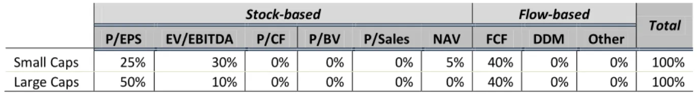
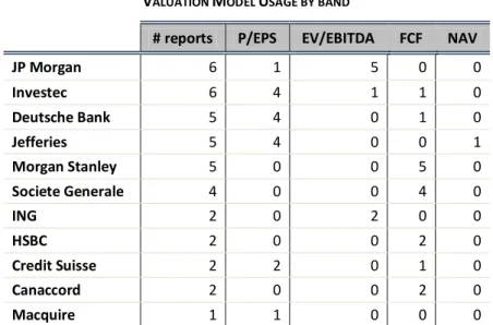
4.4. EMPIRICAL RESULTS ... 31
4.4.1. Descriptive Statistics ... 31
iii
4.5. CONCLUDING REMARKS ... 34
CONCLUSION ... 36
APPENDIX ... 37
iv
II
L
IST OF
T
ABLES
Table 1 - Full Sample Data Treatment... 16
Table 2 - Sub Sample Division... 17
Table 3 - Valuation Errors... 19
Table 4 - Absolute Errors ANOVA Analysis Between Models... 21
Table 5 - Intra-Sample Paired Tests p-value ... 22
Table 6 - Absolute Errors ANOVA Analysis Between Subsamples... 23
Table 7 - Cross Sample Difference in Absolute Valuation Errors... 23
Table 8 - Univariate Regressions... 25
Table 9 - R Squared Values for Univariate OLS Regressions with Different Growth Rates... 27
Table 10 - Small Sample Data... 30
Table 11- Descriptive Statistics... 32
Table 12 - Dominant Valuation Model Used... 33
Table 13 - Total Usage of Valuation Methodologies... 33
v
III
N
OTATION AND
A
BBREVIATIONS
AIG Abnormal Income Growth
Blue Chips Very large companies
BVE Book Value of Equity Book Value of Equity
CAPM Capital Asset Pricing Model
Caps Market Capitalizations
CSR Clean Surplus Relationship
DCF Discounted Cash Flow
DDM Dividend Discount Model
DIV Dividends
DPS Dividends per Share
EBIT Earnings Before Interest and Taxes
EBITDA Earnings Before Interest, Taxes, Depreciation and Amortization
E(DPS) Expected Dividends per Share
e.g. Example Given
EPS Earnings per Share
EV Enterprise Value
FCF Free Cash Flow
FCFF Free Cash Flow to the Firm
FCFE Free Cash Flow to Equity
g Growth Rate
GAAP Generally Accepted Accounting Principles
I/B/E/S Institutional Brokers' Estimation System
IFRS International Financial Reposting Standards
ke Cost of Equity
NAV Net Asset Value
NI Net Income
OJ Ohlson and Juettner-Nauroth
OLS Ordinary Least Squares
P/B Price-to-book Ratio
P/E Price to Earnings Ratio
P/EPSt Price to Period t Earnings per Share
PER Price to Earnings Ratio
vi
Q3 Third Quartile (Below 75th Percentile)
R&D Research and Development
RI Residual Income
RIV Residual Income Valuation
RIVM Residual Income Valuation Model
SD Standard Deviation
S&P500 Standard & Poor's 500 Index
SIC Standard Industry Classification
US United States
USD United States Dollar
vs. Versus
V/P Value to Price Ratio Debt Value
Equity Value
1
C
HAPTER
1
I
NTRODUCTION
Various methodologies of using accounting numbers as a proxy to calculate a firm’s value are broadly used by individual investors and financial companies to analyse and recommend investment opportunities in equity capital. However, since financial research and innovation have become more refined, several debates have been ensued, related to matters such as the specificities, downfalls and practical implementations of each model, and to which method brings the best results for each singular situation.
This paper proposes to appreciate the performance and the usability of different equity valuation methods, between firms with high and low market capitalization. Hence, its core purpose is to compare the results of four valuation methodologies - being two stock-based and the other flow-based ones - attending to how their efficiency, practical utility and limitations change across different firm sizes. Firms with a higher market capitalization are more “on the spotlight” than smaller firms, and thus considered to have more credible and transparent information than smaller firms. Also, the so called “blue chips” are more liquid and have a higher number of daily transactions on stock exchanges around the world, so if the market consensus is considered as the fair price for a certain security, then it would be expected that a higher number of transactions will ensure the company is correctly priced. On the other side, some investors believe that large caps are, in their majority, overpriced due to their popularity and the “crowd effect” it generates. Yet, on this thesis, the market equilibrium price will be considered as efficient in both cases. Throughout this study, it will possible to observe that despite the widely spread support for the flow based models found in the literature, stock based models, in particular the price to earnings multiple, yield a closer valuation output to that equilibrium price. Moreover, despite that superiority being found across all subsamples, significant differences are present between the valuation of high and low caps, with models generally performing better for the prior. Brokerage houses’ equity reports take, up to some extent, this difference in consideration. However, choosing a methodology over the others seems to be mainly influenced by investment bank’s internal practice.
The study will start with a review of past literature, focused on equity valuation using accounting numbers. This first section will present some research already performed on the topic and on the models analysed. Additionally, a brief explanation of the reasoning behind such methodologies will be provided, as well as some advantages and disadvantages discussed in the literature. Next, on Chapter 3, it will be enclosed a large sample analysis, in which the valuation techniques are put
2 to the test on how well they perform. To do this, an industry subdivision is considered on top of the low and high market capitalization dissection, allowing for the comparison between the different methodologies for a total group of ten subsamples. In each of these cases, the models are ranked for every division, and the differences in performance between groups - especially between large and small companies within each industry - are highlighted and documented. In the following section a small sample study is conducted to a set of broker’s reports, in order to examine how the firm size influences the methods used in practice. These reports are analysed individually and selected variables, only viable to be studied in this kind of analysis due to firm-specificity, are considered. Chapter 5 summarizes the main results and core learning, and proposes some additional research on the topic.
3
C
HAPTER
2
R
EVIEW OF
L
ITERATURE ON
E
QUITY
V
ALUATION
U
SING
A
CCOUNTING
N
UMBERS
2.1.INFORMATIONAL CONTENT AND USEFULNESS OF ACCOUNTING NUMBERS
Using accounting numbers as a base to perform an equity valuation is an intrinsic need of developed financial markets. This need is not only a reality for companies, when evaluating and optimizing projects, deciding upon capital structure, and formulating strategic paths, but also for individual investors and analysts, who need to support their investment decisions, recommendations and ratings (Palepu et al., 1999). Even if the efficient market hypothesis may be considered to hold true, it does not necessarily imply that all stocks are correctly priced at a given point in time (Malkiel, 1989). Various methodologies are therefore used by investors to find what they believe to be mispriced securities and opportunities to earn abnormal returns.
There are several methods of performing such equity valuations. One commonly applied distinction is between the entity perspective and the equity perspective. The first one focuses on valuing the company as a whole - or its assets value - and then subtracting the market value of claims other than equity (mainly debt and preferred equity), in order to find the market value of common equity; whereas the second aims at isolating the claim in the firm that is entitled only to its shareholders. While Miller and Modigliani (1958) argue that “(…) the value of the firm should not be affected by the share of debt in its financial structure or by what will be done with the returns – paid out as dividends or reinvested (profitably)” - this is, that capital decisions do not have an impact on the firm value (capital irrelevance theory) - Miller (1977) notes that such argument does not sustain in the presence of taxes.
Another more practical distinction is, according to Damodoran (2002), the grouping into one of the following categories: relative valuation, absolute valuation, returns based valuation and contingent claim valuation. For the purpose of this study, the models used will be divided into either stock-based (market multiples) or flow-based (DCF variations).
However, it is important to bear in mind that valuating companies is not an exact science. This is defended by Lee (1999), according to whom performing a valuation can be seen as much of an art as it is science. The uncertainty about the future flows of a company implies that the best analysts can aim for is an educated guess, rather than a definite true. In fact, the limitation of accounting numbers and, thus, the utility of the data generated are questioned (Canning, 1929; Gilman,
4 1939), supporting the growing amount of regulation and standardization in accounting practices, such as the implementation of GAAP regimes and, more recently, IFRS.
On their ground-breaking paper, Ball and Brown (1968) contest this argument and analyse the importance of accounting figures, as well as its content and timing. Although the authors agree on net income figure limitations - that it derives from a specific set of procedures, and it does not represent a fact unless a specific set of rules is considered - it was found to reflect the majority of the relevant information in a given year. In what concerns to timing of the net earnings announcement, it was found that prices in general reveal anticipation prior to the announcement date, meaning there are other more timely sources of information, such as periodic interim reports and press releases. Another subject attended by the authors is the impact of market-wide information on a firm’s price. They find that in the absence of new firm-specific information, market-wide information accounts for most of the changes in a firm’s price, and that this information represents on average between 30% and 40% of total price variations. Also, upon the study on equity returns on consecutive periods, it is concluded, that a significant negative correlation exists between the return of two consecutive periods. This paper was the first to empirically document the importance of the annual income number.
In line with these findings, Beaver (1968) also uncovers significant price movements relating to earnings announcements, as well as a change in the volume of trade comparing to dates prior to the announcement. A direct implication of this is that the earnings figure has an impact on trading price, especially when weighted against pre-announcement expectations. Yet, the authors' analysis does point out the limitations of using the earnings announcement as the only source of information, namely the availability of more timely sources and the manipulability issues relating to the fact that accounting earnings may focus on a different set of procedures.
Although main literature does not consider the earnings figure as the ideal source of information, there seems to be a consensus about the fact that accounting information does contain some informational value. Moreover, this information is, usually, easily available to investors, making its use so popular and several models have been developed and widely applied to make use of this numbers.
2.2.VALUATION MODELS
As noted by Lee (1999), the value of an equity claim is no more than the discounted value of all future cash-flows arising from it. This theoretical concept is the most widely accepted definition of intrinsic value of an equity security. However, not all models rely on estimating future cash-flows and discount rates (Palepu et. al, 1999). The first type of models presented in this paper are
5 designated as stock-based valuation models, which make use of available information from comparable firms, and apply it as a proxy to perform a valuation. This is by far the simplest to apply method because it does not need a large number of judgments, estimates or assumptions. The other type of models analysed is the flow-based one, often designated as fundamental analysis. These models are usually more complex and its implementation is normally dependent on a high degree of judgment. Conversely, they are supported by a stronger theoretical background, once, and as mentioned by Lee (1999), they rely on an estimation of future variables.
2.2.1. Stock-Based Valuation
The advantage in this kind of valuation is the straightforward process of implementation (Liu et. al., 2002). By far the most common method of stock-based valuation is the market multiples method. Under this method, the analysts assume that the market correctly prices some firms, which are identified as comparable and whose business characteristics are close enough to the company being evaluated. The objective is to use those firms’ value as a proxy to perform the analysis. For this reason, this sort of method is defined as relative valuation by Papelu et al. (2000).
Penman (2003) states that when applying the multiples method it first is necessary to identify the correct comparable firms. Typically this is done by selecting firms with the same type of business, which therefore suffer from the same type of unsystematic risk. The assumption that both the cash flows and the risk profiles of these firms are comparable is a key element on this model. After this peer group is chosen, it is necessary to select a value driver, which is a figure usually from the firm’s financial statements and assumed to be proportional to the firm’s value. The proportion between the selected driver and the firm’s value is called a multiple, and can be defined for a given observation as:
The multiples collected from all the peer group are then averaged and applied to get an estimate, according to the formula:
Different value drivers will, most of the time, result in different estimates. This approach can also be applied at both an equity level and an entity level. Equity multiples aim to estimate only the shareholder’s part of the firm, while entity multiples (also called enterprise-value multiples) predict the value of the entire firm, including other debt and preferred equity. Equity and entity multiples usually use different value drivers.
6
SELECTING COMPARABLE FIRMS
The creation of a peer group can be a difficult task because generally no two companies are alike. An ideal peer group would be composed by companies with the same risk profile, same pattern of cash-flows and similar profitability. In practice, this is an impossible task. One possible solution to this problem would be to choose only one comparable firm. This criteria has the advantage of selecting only the most similar company. However, firm-specific factors and firm-specific risk factors would greatly impact the final valuation. Thus, a recurrently used solution is to pick a number of comparable firms instead. Usually, the chosen firms operate on the same industry, although - and as noted by Penman (2003) - even within the same industry various sub-groups are formed, reducing comparability.
A study by Alford (1992) compares the results obtained with different types of peer group divisions, and determines that using companies with the same 3-digit SIC forms a better peer group than other kind of divisions (including 2-digit and 4-digit SIC). The same conclusion is again reached by Liu et al. (2002).
SELECTING A VALUE DRIVER
The selection of a value driver is very important considering that it greatly influences the valuation outcome. One important factor to have in mind is that some value drivers are affected by leverage, and unless the peer group is composed of firms with the same leverage ratios - which is highly unlikely - results will reflect such impact. Penman (2003), suggests estimating enterprise value, rather than equity value, would be a more correct approach because of this factor.
The paper of Lee et al. (2000) provide a good comparison on the performance of various value drivers across industries and points in time, and ascertains that the same performance ranking between value drivers is kept across time and industries, and that valuations based on future earnings forecasts produced the best results overall. This outcome continued getting better when the forward horizon increased, meaning multiples based on 3 years forecasts (EPS3) performed better than multiples based on one and two years forecasts. Also, earnings drivers were found to outperform book value drivers, whereas sales value shown to be a poor value driver, as well as cash-flow based drivers which scored the worse in the analysis. Another interesting conclusion was that enterprise value multiples performed worse than equity ones, contradicting Penman (2003).
7
THE BENCHMARK MULTIPLE
While computing the benchmark multiple for each comparable firm may be a straightforward process, there has been done some research about the best way to average these observations. One possible way to accomplish it would be by doing a simple arithmetic mean. However, this approach would imply a great impact of outliers in the final multiple and, therefore, a better solution would be to do a weighted-average arithmetic mean, or even to use the median value. Yet, according to Baker and Ruback (1999) and Liu et al. (2002), the method that yields the best results is the use of a harmonic mean, defined by:
Because the harmonic mean is always smaller than the arithmetic, it contradicts some of the upward-based valuation that most multiples calculated by arithmetic mean deliver.
In summary, multiples popularity is connected to their ease of use and fast information availability. It is interesting to note that the best performing multiples are based on analyst predictions, not to present accounting numbers. The use of this methodology does create a new problem by itself. The introduction of an estimated figure - the earnings forecast - not only introduces another variable in the model but also increases the level of complexity and judgment required (for example the decision of which analyst’s earnings prediction to use).
A major drawback of this comparative valuation, according to Damodoran (2002), arises if we challenge the assumption that the comparable companies are correctly priced. In fact, if this is not the case, multiples valuation will be biased to start with.
2.2.2. Flow-Based Valuation DIVIDEND DISCOUNT MODEL
(
DDM)
The Dividend Discount Model sits on the theoretical base that an equity claim’s value is equal to the present value of all future cash inflows resulting from it. This model was first developed by Williams (1938) and had a great acceptance by the academic community.
The DDM valuates an equity claim by discounting the value of expected future cash dividends (E(DPS)) at a given cost of equity (ke), in order to find the present value at time zero ( , or equity value (Ross et al., 2008).
8 The task of estimating dividend payments for a larger horizon is, however, very difficult. In practice, the dividends are usually estimated for a specific horizon, known as explicit period and, after that, the terminal value is calculated by either assuming them to remain constant in perpetuity or to grow at a constant rate (Gordon et al., 1956).
Price per share with constant dividends in terminal value:
Price per share with dividends growing at a rate of g (Gordon growth model):
Despite the intuitive nature of this model, it has some shortcomings. In the first place, it is very difficult to predict the dividend patterns of a company, especially on the long run. Also, there are profitable companies who never paid dividends. A good example of a shortcoming in this method is if the company decides to use its residual income to repurchase common stock. This kind of action has an effect to shareholders’ equity similar to dividend payment, but is not captured by the model. Finally, a limitation of this model resides on one of the assumptions it relies on: the Miller and Modigliani (1961) capital irrelevance theory. According to this theory, the reinvestment of dividends will not alter the firm’s value because they are reinvested at the firm’s cost of equity (ke). However, Fisher (1961) and Black and Scholes (1974) contest this assumption and find out that dividend policy does have an effect on share prices.
Penman (2003) points out the fact that this model works best for stable firms with fixed dividend payout ratios.
DISCOUNTED CASH FLOW MODEL
(
DCF)
The DCF model relies on the same concept as the DDM presented before. The difference between both is that on the DCF case, the value added comes from the free cash flows – amount of cash available after investments have been deducted – instead of dividends. As presented by Damodoran (2002), there are two types of free cash flows: to the firm (FCFF) and to equity (FCFE).
9 The main difference between both formulas is the perspective considered. The FCFF represents the free cash flow available for the firm as a whole, whereas FCFE corresponds only to the free cash flow available for the firm equity owners.
Both these free cash flow measures are discounted at different rates. While the FCFF is discounted at the weighted average cost of capital (WACC) for the firm, the FCFE is discounted at the cost of equity.
Note that the WACC value represents no more than an average of the firm’s cost of capital, weighted by market value. The difference between the first perspective presented and the second will be exactly the market value of the debt for the firm in question.
This model has gained popularity over the DDM because free cash flows are available even for firms that pay zero dividends and because the cash flow measure is not affected by accruals. Shortcomings of this model relate more to its application that it’s theoretical base. On the first place, analysts usually forecast earnings rather than free cash-flows, so additional adjustments are necessary (Damodoran, 2002). Moreover, if there is an especially high or low investment value for the present year, then a longer explicit period must often be considered to avoid making a mistake. As affirmed by Penman (2003), if a firm cuts its investments to zero in a given year, its free cash flow for that year will increase and, unless a longer period is considered to fully capture the effects of that decision, the result will be an increased valuation.
The applicability of this model, although not suffering from as many drawbacks as the DDM, still has its limitations. As it happens with the previous model, DDM will provide better results for firms with stable cash-flow patterns, such as mature firms.
10
RESIDUAL INCOME VALUATION MODEL
(
RIVM)
The residual income valuation model is based upon the principle that the value of a firm’s equity is equal to that firm’s earnings (book value) less the cost of equity based upon the period’s initial book value. It is in fact, as noted by Lee (1996), a model based on the value created during the analysed period, and its economic reasoning comes from the fact that it is a measure of the economic value added.
This model was addressed not only by Ohlson (1995), but formerly by Preinreich (1938), Peasenell (1982), among others. According to O’Hanlon (2009), the model has its base on the clean surplus relationship (CSR):
The concept of abnormal earnings represents the earnings in excess of what would be expected given the firm’s initial period equity value ( ) and a given opportunity cost, or normal return rate, given by the firm’s cost of equity capital (ke). The residual income is therefore represents the earnings in excess of what would be “normal” given the risk profile of the company (Penman, 2003) and is calculated as:
The equity perspective application of the RIVM then becomes:
Ohlson (2005) notes that the intrinsic equity value, given an abnormal growth assumption of zero, equals its book value. Deviations from the price relatively to the book value come from expected earnings higher (or lower) than the opportunity cost. If a company is expected to earn more than the normal return, then the market price will incorporate a premium over the book value. Otherwise, a discount is observed.
The attractiveness of this model comes from the fact that it uses accounting values, addressing some of the implementation issues connected with the other flow models presented before, and also that it incorporates accrual accounting. Courteau et. al (2007) and Penman and Sougiannis (1998) note the superiority based on empirical evidence of the RIVM model compared to the DDM and the DCF, both in accuracy and in explaining stock price movements. Reasons stated are not only the use of book values - and consequently more readily available forecasts - but also the
11 treatment of the investment as an asset, issuing one of the problems with the DCF. Despite that, Lundholm and O’Keefe (2001) find that the value estimate provided by RIVM and DCF are the same when complete statements are available.
However, the use of accounting numbers figures brings its drawbacks. As discussed before, accounting numbers do not have a meaning unless a specific set of rules is considered. Therefore, they are subject to manipulation, which affects the valuation. Ohlson (2005) identifies that despite the model resting on the clean surplus relationship assumption, GAAP earnings constitution is not in accordance with it. Furthermore, as with other earnings based models, it loses accuracy when growing firms with low actual cash flow are considered.
OHLSON AND JUETTNER
-
NAUROTH MODEL(
OJ)
This model was the object of study by Ohlson&Juettner-Nauroth (2005), and it is frequently addressed as the abnormal earnings growth model. As noted by Penman, 2003, it is based on the same conceptual background as the RIVM; however, it tries to address some of the problems with this later model by replacing the current book value of equity with the capitalized earnings from the subsequent period. According to Ohlson (2005) this model is superior to the RIVM because it does not need an anchor on book values and it the clean surplus relationship is not a required assumption. This model is defines as:
This model expresses its premium in incremental earnings adjusted for dividends (O’Hanlon, 2009). Because net income can be defined as:
Then this model captures a larger piece of the intrinsic value when compared to the RIVM, diminishing the weight of the terminal value. Furthermore, Ohlson (2005), finds the capitalized future income to be a best approximation of market value than book values.
One advantage of this model is that it focuses on earnings growth rather than on book value growth. However, as noted by Penman (2003), the correct application of this model is dependent on the understanding of accrual accounting, because forecasts’ quality depends on it.
12
2.2.3. Empirical Evidence on Model Performance
There is no universal consensus about which valuation technique brings the best performance. One important debate is regarding flow based and stock based methods. While the first ones have the support of academics and a more intuitive reasoning behind them, they are far less used than the later.
Regarding the stock based models, an important research on their performance was made by Liu et. al (2002). In this paper the performance of different types of value drivers are compared, using different peer groups and calculation methodologies. The authors of this study, however, recognize its limitations: by excluding firms with negative multiples, the final outcome will be positively skewed, and some emerging firms with negative cash-flows will be excluded from the analysis. The results are nevertheless informative and useful, especially when considering its applicability for firms with more stable cash flows. Multiples based on forward earnings were found to perform reasonably well, and to explain most of the stock prices, while cash flow and sales multiples performed worse than what would be expected. Furthermore, the authors used both the harmonic mean and the median, in order to maintain comparability with previous studies, but found the harmonic mean measure to outperform the median, as found by Baker and Ruback (1999). Regarding the peer group selection, the study also concluded that the performance of a given multiple can be improved by selecting only firms from the same industry. One interesting result is that the ranking between multiples was not altered between industries, contradicting the work of Tasker (1998).
Flow based models’ comparability has been the object of diverse studies, such as Kaplan and Ruback (1995), Bernard (1995), Penman and Sougiannis (1998) and Francis et al. (2000). This later one focuses on the payoffs of selected portfolios but extends the analysis to a comparison between the DDM, DCF and RIVM. This later model was found to perform superiorly, with the authors arguing that the usage of book value and residual income created a smaller error than the one created by the growth rate and free cash flow/dividends forecasts. Based on this model, Frankel and Lee (1988) show that an estimated value to price ratio is a very good predictor of long term returns and even construct a portfolio where, by buying high V/P stocks and selling low ones, it was possible to achieve a return far superior to the market average in the period analysed. Furthermore, this V/P ratio also showed to be superior at explaining cross-sectorial prices than the price to book multiple.
It is however important to note that there is not much literature about the relative performance of the OJ model, because the work of Ohlson and Juettner-Nauroth regarding it did not come out until 2005.
13 Literature arguments in favour of flow based models can be found in Gleason et al. (2008), who find that discrepancies between estimated values and price are more related to unreasonable assumptions and estimates than to model errors. Courteau et al. (2007) compare these models to multiples and finds them superior in both current price accuracy and return prediction, although they also find both techniques can be combined for even better results.
Despite all the academic arguments, Baker (1999), through a series of surveys, comes to the conclusion that the price to earnings multiple is by far the most commonly used model, while the flow based models are of little importance to analysts. Bradshaw et al. (2006), attributes that fact to the higher number of buy recommendations that can be supported by the P/E market multiple. Demirakos et al. (2004) readdress this issue by studying broker’s reports on three different industries for 104 different firms. Their results are in line with Baker (1999), finding that relative valuation, especially the P/E ratio, is still the most used. Moreover, between the flow-based models, the DCF model is preferred to the RIVM and to the DDM. Analysts who use both types of valuations to support their recommendations usually prefer relative valuation as their main model. However, analysts do tend to vary valuation models used according to the industry or sector they are working on, e.g. Demirakos et al. (2004), found that on the beverage sector (a mature industry with more stable cash flows), there is an increase in the usage of the price to cash flow multiple.
On the next section, these models will be compared in how well they perform when applied to firms with a high market capitalization - also called "blue chips" - and to smaller firms.
14
C
HAPTER
3
L
ARGE
S
AMPLE
A
NALYSIS
3.1.RESEARCH QUESTION AND BRIEF REVIEW ON RELEVANT LITERATURE
As previously discussed on the literature review of this paper, several are the factors that influence model’s performance and reliability. The research question of this paper will focus on how these valuation techniques perform when used for companies with a high market capitalization, often known as blue chips, in contrast to low market capitalization firms.
This distinction between big and small has been subject to analysis from various academics on the past. As noted by Lee, T. (2008) in a report named “The Value in Small Caps”, investing in large caps is often preferred by the investments due to a conjunction of several factors. First of all, the perception of increased safety is often used as an argument over blue chips. The argument “too big to fail”, which brought a lot of debate in the 2008 financial crisis aftermath, is still used to highlight the higher perceived safety of larger firms. Another argument is that small stocks may not be very liquid because they are not transitioned nearly as much as larger ones. This leads to a possible mispricing, difficulties to buy or sell the stock and a possible increase in transaction costs. Moreover, the small stocks are usually more sensitive to economic conditions and therefore bear higher volatility. This later argument is often contradicted by portfolio diversification theories, which argue that unsystematic risk (or firm specific risk) can be diversified away. Finally, there are concerns related to information asymmetry and reporting quality. Because larger firms are more on the radar of regulators, it is perceived that a higher reporting quality is demanded of them, with less room for error. In practice, there has been some large scale reporting scandals that shocked the investment world (e.g. Enron), putting on stand the validity of these concerns.
The attractiveness of large stocks for investors must, however, be weighed against the increased profitability of small capitalization firms over the last decades. Fama and French (1993), proposed a three factor model to replace the CAPM cost of capital, where they incorporate a firm size factor. According to their research, smaller firms have yielded higher returns, which must be a factor in calculating the required return for a given equity claim. Carhat (1997) goes even further proposing a four factor model, but his work also confirms the relevance of market capitalization as a factor influenced return. Lee (2008) also found that from the period from 1993 to 2008, the small market capitalization firms have generally outperformed larger ones. Yet, this report contests the concept that low caps have a higher downsize risk. Once analysing the recessions during this period, the author ascertains that while on economic expansion small firms
15 had higher returns, during a recession the returns were approximately the same for both kinds of firms. Moreover, regarding relative valuation, the report states that small caps have lower price to book multiple than the larger companies, which implies low valuation levels. Moreover, based on the same multiple, small caps are traded at a 40% to 50% discount in relationship to their larger counterparts.
In this section, the study will focus on valuation accuracy and bias for a large sample dataset, using four of the models previously analysed. While the comparison of returns depending on the market capitalization will not be directly tested, it will have an impact on the relative value of estimates because it is a factor incorporated in each firm’s trading price.
3.2.VALUATION MODELS USED
This analysis comprises only equity perspective valuation models, two stock based and two flow based. The stock based models chosen were the two best performing models in the literature review section, the price to expected earnings in period 2 (EPS2) and the commonly used price to book. As far as flow based models go, the RIVM and OJ models will be analysed. The RIVM was found to be the best performing model according to the literature, while the OJ model aims to be an improvement over the RIVM. However, not many relevant empirical studies have been performed on the later, considering its proposal has been relatively recent.
3.3.
RESEARCH DESIGN3.3.1. Data
The raw data used to perform this analysis was obtained from the Compustat and I/B/E/S databases and comprises 10.432 observations from US publicly traded common stocks relating to non-financial institutions, with stock prices of at least 1 USD. All the firms analysed are followed by at least one analyst and each observation relates to the fiscal year ending in December of each year, from 2006 to 2011.
While Compustat data is mostly collected directly from the firm’s financial statements from the period on 31st December, I/B/E/S gathers data from analyst forecasts and reports, on the 15th of
April, date in which the valuation of this analysis will occur. An important difference between the firms’ data and the analysts’ figures is that on the later, earnings are not defined as in the GAAP regimes, but rather as sustainable (or recurring) earnings. Moreover, while I/B/E/S data is adjusted for stock splits and dividends, Compustat is not. Therefore, an adjustment factor was
16 applied to Compustat data in order to assure consistency in the number of shares and shares based measures (such as EPS).
From the initial sample, various observations were discarded by not fulfilling the requirements to perform the analysis. This process is summarized on Table 1:
From the initial data of 10.432, a final number of 7379. Firms with missing or negative earnings were excluded because the relative valuation would be either meaningless or impossible. The same reasoning applied to book value. Moreover, the analysis performed required a peer group, chosen from the 2-digit SIC code. Because the models based on multiples exclude the firm’s own value, observations that had the only SIC code for a given year were excluded.
Additionally to the described, firms with negative or non-available betas (totalling 38 observations) were assumed to have the same beta as the industry average. This adjustment was done given negative betas have no economic reasoning because they imply a negative impact of the risk premium on the required return.
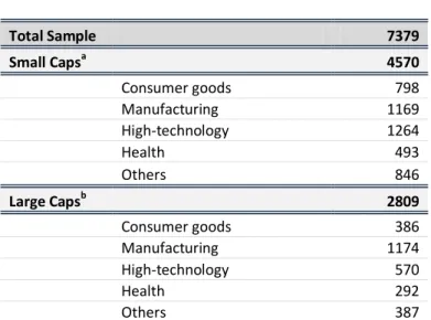
Furthermore, the sample was divided according to the definition of the federal reserve of firms with small market capitalization. According to it, firms with less than two billion market capitalization are considered small caps, firms with market capitalization between two and ten billion are medium caps and firms with more than that are considered large caps. Because the data had much more observations below two billion than in any of the other groups, only one division was made: small and big market capitalizations. Furthermore, the focus of this analysis was also the comparability of this results in a cross-industry basis, so a further division was made, according to the companies’ 3-digit SIC codes, into five different activity sectors. This division was suggested by French (2012) and divides companies in one of the following businesses: consumer goods, manufacturing, high-technology, health and others.
TABLE 1
FULL SAMPLE DATA TREATMENT
Initial Data 10432
Excluded:
Negative or zero earnings -2441
Non available earnings -300
Negative or no Book Value -291
No peer group -21
Total 7379
17 In addition to the presented data, the Bloomberg database was used to extract market returns and bond returns. The S&P500 return for the 20-year period finishing in 2007 averaged 10,496% annually, and was used as the market return. This period was chosen because it excludes the 2008 financial crisis, which would cause an excessive negative skew of the average return. Bond yields selected to perform the analysis correspond to the 10-year US bonds yields, on each year. This values range from 4,702% to 2,212% and are used as each year’s risk free rate.
3.3.2. Model Implementation
STOCK
-
BASED MODELS(
MARKET MULTIPLES)
The implementation of the two drivers chosen (earnings estimate for period two and book value) was done in similar fashion. Following the results of Baker and Ruback (1999) and Liu et al.(2002), the method for calculating the average multiple used was the harmonic mean, because it is described in these studies as outperforming the other methodologies. Despite Alford (1992) noting that a division based on the 3-digit SIC code yields the best results, the 2-digit code was used instead to avoid excluding more observations from the sample because of an absence of peer group. Each peer group was computed only for observation of the same year, to avoid using the same peer more than once and because this analysis makes sense only for given market conditions that are present at a given point in time. For the price to EPS2 multiple, an average of analyst estimates for period two was considered as the value driver. No negative equity values resulted from the implementation of these models due to the exclusion of firms with negative earnings estimates and book values.
TABLE 2 SUB SAMPLE DIVISION Total Sample 7379 Small Capsa 4570 Consumer goods 798 Manufacturing 1169 High-technology 1264 Health 493 Others 846 Large Capsb 2809 Consumer goods 386 Manufacturing 1174 High-technology 570 Health 292 Others 387
Table 2 summarizes final sub-sample sizes; a Small Caps consider
solely firms up to 2 billion; b Large Caps consider solely firms larger
than 2 billion
Note: Table summarizes final sub-sample sizes; a) Small Caps consider solely firms up to 2 billion; b) Large Caps consider solely firms larger than 2 billion
18
FLOW BASED MODELS
The RIVM model was computed using a two-year period based on the average analyst estimate for earnings, and the residual income formula described in the literature review section. Furthermore, as in the model stated by Frankel and Lee (1998), a growth rate was applied in the terminal value. This long-term growth was initially assumed as 2%, an assumption that will be challenged later on this paper. The value estimated provided by the RIVM is therefore equal to the sum of the year zero book value, the actualized residual income value for periods one and two and the actualized terminal value, a growing perpetuity of the second year residual income. The OJ model’s formula presented earlier was used to compute this model for each observation. A one period estimate of the abnormal earnings growth was used, and the abnormal earnings growth computed from one year average analysts’ earnings estimate for 1 year and 2 year ahead EPS. Next year’s earnings per shares were capitalized and added to the intrinsic value calculation. The terminal value was computed as the capitalized perpetuity of the abnormal earnings growth with no growth in the perpetuity. This assumption comes from the theory that in perpetuity, abnormal earnings growth ceases to exist due to the increasing competition, and will be revised later when a robustness test is performed.
The cost of equity used for both of these methodologies was the same, computed by using the capital asset pricing model with the 10-year US government bonds as the risk-free rate and the 20-year S&P500 returns as the market return. This formula can be defined as:
With ke being the equity discount rate, rf as the risk-free rate, as the company’s observed beta and the relationship rm-rf representing the market risk premium.
This methodology yielded some negative results in the RIVM model when the expected earnings for periods one and two were smaller than the equity’s opportunity cost (represented by . Because negative equity values cannot happen in the real world, a total of 87 negative observations were trimmed to the value of zero.
3.4.EMPIRICAL RESULTS
3.4.1. Descriptive Statistics
In order to compare the results from the application of the models studied, the same methodology was applied as in the papers of Francis et al. (2000), Liu et al. (2002) and Courteau et al. (2007),
19 using market prices as a benchmark and calculating two types of errors: signed and absolute prediction errors.
Signed valuation errors represent the tendency to over or under evaluate because it allows for negative values; it is therefore known as model bias. Absolute prediction errors are a measure of the model’s accuracy. While it does not allow for negative values, it represents the percentage of a firm’s market price that is not incorporated in the value estimations.
20 As it is possible to observe on Table 3, the price to earnings multiple presents not only the smaller valuation bias, but also the highest accuracy. In fact, for the full sample and the small caps, the signed prediction errors on this model are not significantly different from zero at a 5% level, showing this model has a low tendency to under and over evaluate the company when compared to the market price. Interesting to see that on a first look, the stock based models seem to be outperforming the flow based methodologies across the board. However, this will be tested more in debt forward on this paper. It is important to note that although the price to book ratio has the second lowest signed prediction error for these three cases, its absolute prediction errors are usually among the highest. This may indicate large positive and negative errors that are balancing each other out. This seems to be the case because this model presents not only high values for standard deviations, but also very distant 1% and 99% percentiles. Also a value to be noted is the -1 that the RIV model presents on the 1% percentile of both the full sample and the small caps subsample. This value represents the smallest possible outcome for the ratio , happening only when the value estimate is zero. The explanation for this is the previously mentioned adjustment of negative equity values to zero, which caused a considerable number of these observations. As expected, the flow based models seem to be performing relatively better for the large caps than for the small market capitalization firms.
It is also relevant to point out that the median values for the signed prediction errors are, for the great majority, negative values. This leads to the conclusion that the models, once based on accounting numbers, are failing to capture some of the sources of value, such as brand image and company reputation.
On the analysis for all the subsamples, these results seem to be confirmed. Note that for the health industry, especially between low cap firms, the relative valuation models seem to be performing remarkably well. Also, it is interesting to see that the price to book ratio has the lowest signed error on the consumer goods companies with a low market cap. However it has the highest absolute prediction error, in line with the conclusions drawn before. The price to earnings multiple is, across all industries, the one with smaller (closer to zero) signed and absolute errors. It is important to note that, as exposed by Damodoran (2002), although analysing the mean and the median should almost always bring the same results, the median is considered to be a more stable indicator, and therefore most tests presented from this point on focus on comparing medians rather than averages.
21
3.4.2. Intra-Sample Analysis
This section will focus on the comparison between how the models perform inside the entire sample and within each sub-sample. In order to do this comparison, three distinct types of analysis were performed. On the first place, an ANOVA table was constructed in order to verify if there is significant statistical difference between at least one of the models in comparison to the other three. Using this testing methodology, the null hypothesis that all the models perform equally in each subsample (for a given market cap and industry category) is put to the test, and were rejected if at least one of these models’ errors were found to be statistically different from the others. Following that, both the paired t-test for the means and the Wilcoxon sum rank test for the medians were performed for each pair of models to test if that difference exists individually.
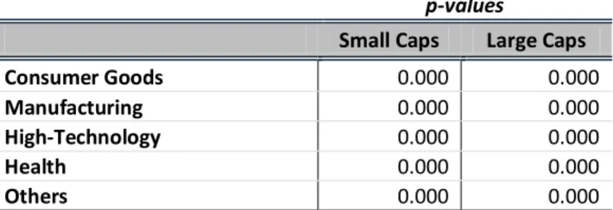
From the ANOVA analysis, represented on Table 4, one would conclude that independently of the industry and the size of the firms considered, there are always significant differences between the accuracy of the valuation models at any given significance level higher than 0%. Therefore, the accuracy of the valuation will depend on the model selection.
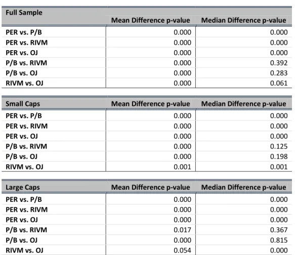
To test the models in pairs, both the Wilcoxon rank sum test and the paired t-test were used, and as it is can be verified on Table 5, by observing the low p-values, the PER multiple produces absolute errors that are always statistically different from the other presented models. This result is in line with the previous analysis which identified the PER as being by far the model that yielded the best results overall. Another result is that, for the median Wilcoxon test, the pairs P/B and RIVM, and P/B and OJ are never statistically different from each other, proving these methods’ errors are in fact very similar. The test to the RIVM and OJ pair is rejected for both the median in the full sample and the mean in the large caps subsample. This result, however, is influenced by the different terminal value growth rate assumptions.
TABLE 4
ABSOLUTE ERRORS ANOVAANALYSIS BETWEEN MODELS
p-values
Small Caps Large Caps
Consumer Goods 0.000 0.000
Manufacturing 0.000 0.000
High-Technology 0.000 0.000
Health 0.000 0.000
Others 0.000 0.000
Table 4 results from ANOVA analysis; P-value of less than a chosen significance level – the 5% level is often considered – means that at least one of the medians of the absolute prediction errors is significantly different from the others.
22 The results for the industry subdivision (see Appendix 2) are in line with the ones for the full sample. While the P/B vs. RIVM is the pair that is more often statistically similar, the absolute errors of these two models are statistically different in some industries, as it is the case of manufacturing and high-technology, for both small and large caps. Also to note is the fact that in the high technology factor, the RIVM and the OJ model, despite the different terminal growth assumptions, are statistically similar.
3.4.3. Cross-Sample Analysis
While in the intra-sample analysis the objective was to find out if there are differences between the models in each subsample, the focus of this analysis is to find out if these models perform equally for all the subsamples.
TABLE 5
INTRA-SAMPLE PAIRED TESTS P-VALUE
Full Sample
Mean Difference p-value Median Difference p-value
PER vs. P/B 0.000 0.000 PER vs. RIVM 0.000 0.000 PER vs. OJ 0.000 0.000 P/B vs. RIVM 0.000 0.392 P/B vs. OJ 0.000 0.283 RIVM vs. OJ 0.000 0.061
Small Caps Mean Difference p-value Median Difference p-value
PER vs. P/B 0.000 0.000 PER vs. RIVM 0.000 0.000 PER vs. OJ 0.000 0.000 P/B vs. RIVM 0.000 0.125 P/B vs. OJ 0.000 0.198 RIVM vs. OJ 0.001 0.001
Large Caps Mean Difference p-value Median Difference p-value
PER vs. P/B 0.000 0.000 PER vs. RIVM 0.000 0.000 PER vs. OJ 0.000 0.000 P/B vs. RIVM 0.017 0.367 P/B vs. OJ 0.000 0.815 RIVM vs. OJ 0.054 0.000
Table 5 presents results from Wilcoxon rank sum test and the paired t-test, to test models in
pairs; The p-values for these tests are presented in Table 4 and in greater detail in Appendix 2 (with the industry sub-samples included).
Notes: Table presents results from Wilcoxon rank sum test and the paired t-test, to test models in pairs; p-values for these tests are presented in Table 4 and, in greater detail and including the industry sub-samples, in Appendix 2
23 For large caps, it is possible to reject the null hypothesis that all the models perform similarly independently of the industry in analysis. In small caps, however, the P/B and RIVM models reject the null (at the 5% level) that there is a difference between the model application in the industries analysed.
As far as signed prediction errors go, only the paired t-test failed to show a difference in the average of these errors for the PER multiple between small and large caps. In all the other models, the division between small and large cap firms seems to have an impact on the signed errors. For the absolute prediction errors, the only non-significant difference is in the average of the price to book multiple model. Note that in the medians, considered to be the most stable measure, there is always a statistically significant difference between small and big firms. Note that for relative valuation the average benchmark multiples between large and small caps vary significantly. In fact, in both the PER and the P/B ratios, the large caps have a higher multiple value, meaning that for the same level of earnings and book values, the value prediction will be higher for the high capitalization firms, in line with the results shown in the literature review section.
Appendix 3 shows the analysis above, performed at an industry basis rather than for the entire sample. It is interesting to note that at an industry level, the differences between valuation
TABLE 6
ABSOLUTE ERRORS ANOVAANALYSIS BETWEEN SUBSAMPLES
p-values
Small Caps Large Caps
PER 0.000 0.000
P/B 0.077 0.000
RIVM 0.111 0.000
OJ 0.000 0.000
Notes: Table presents both the mean paired t-test and the Wilcoxon median rank sum test for the errors of the models between small and large cap firms
Notes: Table synthesizes the p-values of the ANOVA analysis for the test H0: each model performs equally for each industry
24 models detected in the full sample analysis continue to be present. In the manufacturing industry, the p-values of the absolute errors are always close to zero, rejecting the null hypothesis. However, this is not always the case in the other industries. In the consumer goods industries, the RIVM model produces signed errors that are similar between small and large caps, and the P/B’s absolute errors are also statistically similar (with the median test), meaning this model’s accuracy is not dependent on the size of the firm we are analysing. In the high technology industry, there are statistically different absolute errors for only one model, the PER multiple. In the industry group designated by “others”, the RIV model is the only model that does not present a difference between high and low caps. A particularly interesting industry in what concerns these tests is the health industry. In this sector, all the models present p-values higher than 5% for at least one kind of errors, meaning this is the industry where the division between low and high market capitalization less influences the accuracy of the valuation in relation to market value. Also a relevant fact is that the PER model is, across all industries, the more size sensitive model. In fact, the null hypothesis was always rejected for this model’s absolute errors in any of the 5 industries.
3.4.4. Univariate Regressions and Explanatory Power of the Models
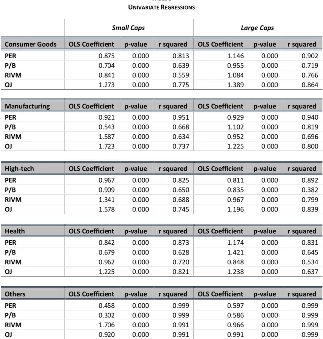
The results presented next regard the OLS regressions performed. The objective of this analysis is to provide an insight of the explanatory power of each model (represented by the ) for the four valuation models and across all the subsamples considered. The regressions performed use only a single variable (the model’s value estimate) as the independent variable, and the market price on 15th of April as the independent one. Also, the regression was done with no constant, according to
the formula:
Because the regressions performed are univariate, the does not need to be adjusted for comparison between regressions. Attending to Table 8, that summarizes the results of the performed Univariate Regressions, it is observable that the p-values are all zero, meaning the explanatory power of the model estimates on the observed price is always statistically significant, as expected. A meaningful result concerns to the industry denominated by “others”.
25 Here, the models have a higher explanatory power than in any other sector, with always above 0,99. This high explanatory power is not explained by a large number of observations because, according to the division explained earlier, this is not the sector with the highest number of observations.
In all the subsamples, the PER ratio is the one that has the highest explanatory power, followed by either the OJ model or the price to book. This ranking often changes when the small and large market capitalization factor is introduced. The P/B model, although it explains a large portion of the price in some industries, scores remarkably bad in the high market capitalization high-tech firms, maybe because these firm’s intrinsic value is not so dependent on their book value.
TABLE 8 UNIVARIATE REGRESSIONS
Small Caps Large Caps
Consumer Goods OLS Coefficient p-value r squared OLS Coefficient p-value r squared
PER 0.875 0.000 0.813 1.146 0.000 0.902
P/B 0.704 0.000 0.639 0.955 0.000 0.719
RIVM 0.841 0.000 0.559 1.084 0.000 0.766
OJ 1.273 0.000 0.775 1.389 0.000 0.864
Manufacturing OLS Coefficient p-value r squared OLS Coefficient p-value r squared
PER 0.921 0.000 0.951 0.929 0.000 0.940
P/B 0.543 0.000 0.668 1.102 0.000 0.819
RIVM 1.587 0.000 0.634 0.952 0.000 0.696
OJ 1.723 0.000 0.737 1.225 0.000 0.800
High-tech OLS Coefficient p-value r squared OLS Coefficient p-value r squared
PER 0.967 0.000 0.825 0.811 0.000 0.892
P/B 0.909 0.000 0.650 0.835 0.000 0.382
RIVM 1.341 0.000 0.688 0.967 0.000 0.799
OJ 1.578 0.000 0.745 1.196 0.000 0.839
Health OLS Coefficient p-value r squared OLS Coefficient p-value r squared
PER 0.842 0.000 0.873 1.174 0.000 0.831
P/B 0.679 0.000 0.628 1.421 0.000 0.645
RIVM 0.962 0.000 0.720 0.848 0.000 0.534
OJ 1.225 0.000 0.821 1.238 0.000 0.637
Others OLS Coefficient p-value r squared OLS Coefficient p-value r squared
PER 0.458 0.000 0.999 0.597 0.000 0.999
P/B 0.302 0.000 0.999 0.586 0.000 0.999
RIVM 1.706 0.000 0.991 0.966 0.000 0.999
OJ 0.920 0.000 0.991 0.991 0.000 0.999
Table 8 summarizes the results of the performed Univariate Regressions. Notes: Reported values result from the regression: Pi = λ*0+λ1*Vi+Ei, with Pi = Observed market price and
26 Note also that with the exception of the health industry, flow based models perform better for large caps than for small caps. A theory for this is that some small cap firms are companies in the growing process, and therefore have small short-term forecasted earnings. A possible solution to better capture the value of these firms would be to either use a larger explicit period, or to readjust the long term growth of the models to capture this effect. Moreover, it is possible to notice a tendency for the OJ model to explain more of the market price than the RIV model.
3.4.5. Robustness Test
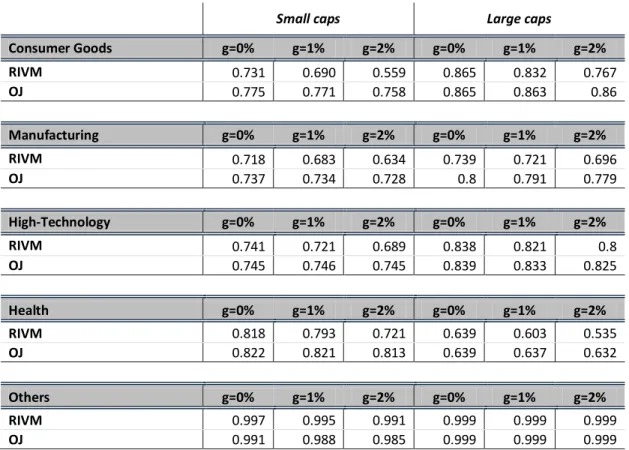
The objective of this analysis is to challenge the long term growth assumptions used to compute value estimates on the flow based models. So far, the RIV model was computed using an assumed long-term growth rate of 2% and the OJ model’s abnormal income growth was theorized to disappear in the long run and therefore the long term growth assumed zero. On this section, three growth rates will be analysed and compared for both of this model: 0%, 1% and 2%. The reason higher long-term growths were not considered is that the denominator (ke-g) would become negative for too many of the observations in the sample.
Appendix 4 shows the descriptive statistics for the three different rates in all the subsamples. It is possible to note that the ranking between both models does not change with the change in the growth rate assumption. The OJ model’s valuation errors are, in the majority of cases smaller than the ones for the RIV model, keeping the previous rank between these two methodologies unchanged. Moreover, and as expected, an increase/decrease in the growth rate assumption will not increase/decrease the performance in the same way for all the industries. While the errors in some sectors are smaller with a 2% growth assumption, in others the 0% value yields the best results. The division between small and large market caps seems to affect the optimal growth rate for the RIV model. In three industries (manufacturing, health and others), the model performs better with a 0% growth rate for low market caps, but for high market capitalization firms, the best results are achieved with a higher rate. Another result that can be drawn from this analysis is that the growth rate assumption that minimizes errors for the OJ model is always 2% in this sample; this result holds both for signed and absolute errors.
It is possible to verify the OJ model, for every assumption and in every subsample, always presents a higher explanatory power than the RIVM model. The 0% growth rate assumption yields the highest explanatory power across industries and in both small and large caps. Also, in line with the results observed earlier, the models always explain more of the price for large market capitalization firms, with the exception of the health industry. Finally, it is interesting to note that RIVM model’s explanatory power is much more affected by the growth rate assumption than the OJ model.
27
3.5.CONCLUDING REMARKS
The results presented in this sector show that the quality of a valuation highly depends on the size of the company, as well as on its industry and the chosen model. The 2-year forward PER performed better across all analysed subsamples, followed by either the OJ model or the price to book value, this later one which performance seems to be highly dependent on the industry being analysed. Moreover, the OJ model, a derivation from the RIVM, was found to perform better than the RIVM, confirming the results of Ohlson (2005).
Finally, it is important to highlight some of the limitations of this study. An obvious shortcoming is the use of April 15th market prices and 31st December reports. In fact, the presence of relevant
news between both dates is being ignored. Also, in the flow-based models, the quality of the model is dependent on the quality of the earnings forecasts as well as on the discount rate. The challenge of those two variables is out of the scope of this paper. Moreover, another limitation is the explicit period used. The accuracy of the valuation may increase with a longer explicit period
TABLE 9
RSQUARED VALUES FOR UNIVARIATE OLSREGRESSIONS WITH DIFFERENT GROWTH RATES
Small caps Large caps
Consumer Goods g=0% g=1% g=2% g=0% g=1% g=2% RIVM 0.731 0.690 0.559 0.865 0.832 0.767 OJ 0.775 0.771 0.758 0.865 0.863 0.86 Manufacturing g=0% g=1% g=2% g=0% g=1% g=2% RIVM 0.718 0.683 0.634 0.739 0.721 0.696 OJ 0.737 0.734 0.728 0.8 0.791 0.779 High-Technology g=0% g=1% g=2% g=0% g=1% g=2% RIVM 0.741 0.721 0.689 0.838 0.821 0.8 OJ 0.745 0.746 0.745 0.839 0.833 0.825 Health g=0% g=1% g=2% g=0% g=1% g=2% RIVM 0.818 0.793 0.721 0.639 0.603 0.535 OJ 0.822 0.821 0.813 0.639 0.637 0.632 Others g=0% g=1% g=2% g=0% g=1% g=2% RIVM 0.997 0.995 0.991 0.999 0.999 0.999 OJ 0.991 0.988 0.985 0.999 0.999 0.999
Table 9 presents the 2 for subsamples under the three different assumptions.
Note: Table presents the R2 for univariate regression of subsamples under the three different growth rate
28 for both the RIV and OJ models, but due to data limitations (limited number of medium-long term forecasts), a two-year period was used.