1 ACCOUNTING
CORPORATE FINANCING CHANGES: CONSEQUENCES FOR DISCRETIONARY ACCRUALS
ESTIMATION
Jorge Manuel Afonso Alves
Escola Superior de Tecnologia e Gestão do Instituto Politécnico de Bragança / UNIAG / OBEGEF
Campus de Santa Apolónia – 5301-857- Bragança / Portugal
Tel:00.351.273 303 121; Fax:00.351.273 313 051
E-mail: jorge@ipb.pt
José A. C. Moreira
Faculdade de Economia da Universidade do Porto / CEP.UP / OBEGEF
Rua Roberto Frias - 4200-464 Porto / Portugal
Tel: 00.351.225 571 272; Fax: 00.351. 225 505 050
E-mail: jantonio@fep.up.pt.
ABSTRACT
This study discusses the impact of financing changes on accruals models and discretionary accruals estimates. It pursues a
threefold objective. Firstly, to show analytically how the occurrence of such changes affects discretionary accruals
estimation. Secondly, to analyse empirically whether different accruals models (Jones, (1991); Dechow and Dichev, (2002);
and McNichols,(2002) reflect in a similar way the impact of changes in corporate financing. Thirdly, to test an existent
solution in literature to mitigate the problem caused by financing changes on discretionary accruals estimates. Empirical
evidence shows that the measurement error induced by not well-specified accruals models is affected by the sign of financing
changes, being different for positive and negative changes; all models reflect in a similar way the impact of changes in
corporate financing and, for the Portuguese context, the matched-firm approach on financing changes used by Shan et al.
(2010) to mitigate the problem caused by financing changes on discretionary accruals doesn’t work well.
K
EYWORDS:
Accruals models, financing changes, SME, Portugal
1.
INTRODUCTION.
The literature is prolific in studies on earnings management (e.g., Ronen and Yaari, 2008). In most cases, they use discretionary accruals as a proxy for earnings manipulation, estimated with a model where accruals are the dependent variable and the firm’s change in revenues (e.g., Jones, 1991) or cash flows (e.g., Dechow and Dichev, 2002) are the main independent variables.
2 Same studies have attempted to find solutions to solve the problem caused by omission of explanatory variables in accruals models (e.g., Dechow et al., 2012;Shan et al., 2010). However, the application of the presented solutions is not always possible to all cases. This happens, for example, with the solution presented by Dechow et al. (2012), according to which we need to know exactly the periods in which accruals are managed and reversed. Gerakos (2012) recognize that such approach is only applicable when working with samples of firms with known manipulation. Other solutions, as the matched-firm approach presented by Kothari et al. (2005), only mitigates the misspecifications for samples where the omitted variable presents extremes values, but can exaggerate misspecification in other situations (Dechow et al., 2012).
One study that is similar to this was developed by Shan et al. (2010), but is based in a different context and use another methodology. According to Dechow et al.(2010), the measurement error in estimating discretionary accruals will have to be related to industry characteristics and the contexts where firms operate. Thus, it’s expected that the solution adopted by Shan et al. (2010) doesn’t work in our context. We will replicate the methodology used by Shan et al. (2010) to demonstrate it’s applicability or not in our context.
Thus, the main reason that lead us to develop this study is because there are recent studies that had analysed the new approaches of estimation discretionary accruals (e.g., Gerakos, 2012;Marai and Pavlović, 2014), which recognise the importance of new evolutions and the necessity to improve the estimation models.
It has a threefold objective. Firstly, to show analytically how the occurrence of such changes affects discretionary accruals estimation. Secondly, to analyse empirically whether different accruals models (Jones, (1991); Dechow and Dichev, (2002); and McNichols,(2002) reflect the impact of changes in corporate financing in a similar way. Thirdly, to test if methodology used by Shan et al. (2010) it’s enough to mitigate the problem caused by financing changes on discretionary accruals estimates in our context.
Although Shan et al. (2010) study was performed under a different economic context and using a distinct methodology, based on its results it is possible to formulate a general expectation that the above mentioned models are not well-specified and suffer from an omitted variable bias.
The empirical methodology adopted is similar to that used by Moreira (2009), based on a comparative static approach. Two versions of each model are estimated, and they differentiate by the consideration in one of them of a variable controlling for financing changes. The differential measurement error allows conclusions about the quality of the model specification and its consequences for accruals estimation. In a first moment a graphic analysis is carried out; afterwards, and to test the robustness of the results, an analysis based on simulations takes place (e.g., Dechow et al., 1995;Hribar and Collins, 2002;Kothari et al., 2005;Shan et al., 2010). We replicate the methodology used by Shan et al. (2010) to see if it’s enough to mitigate the problem caused by financing changes on discretionary accruals estimates in our context. The evidence supports the initial expectations, showing that the analysed models are not well-specified and lack a control for changes in corporate financing.
Two main findings of our study are highlighted: i) estimation errors occur regardless of financing changes size; ii) the measurement error is affected by the sign of financing changes; iii) the methodology used by Shan et al. (2010) to mitigate the problem caused by financing changes on discretionary accruals estimates in our context does not apply.
The present study makes three main contributions to the literature. First, it shows that the measurement error induced by poor specification is affected by the sign of financing changes. Second, the measurement error exists regardless of the size and sign of those changes. Finally, the results of the study add to the literature on the estimation of accruals in a context of non listed small and medium firms and shows that matched-firm approach on financing changes used by Shan et al. (2010) does not apply.
The study contains five additional sections. The second section discusses analytically the accruals impact arisen from financing changes. The following section introduces the methodology to be used and some descriptive statistics. The empirical results are presented and discussed in section four. Finally, the main conclusions, contributions and limitations of the study are discussed.
2. CORPORATE FINANCING CHANGES AND ACCRUALS MEASUREMENT ERROR. 2.1. Accruals definition and its correlation with financing changes.
A balance sheet definition of total accruals (ACC) is as follows (e.g., Dechow et al., 1995;Healy, 1985;Jones, 1991;McNichols, 2002): ACC = ∆CA − ∆CL − ∆CASH + ∆CMD − DA (1) where the symbol ∆ stands for change, CA is current assets; CL is current liabilities; CASH is cash; CMD is current maturities of long-term debt; and DA is the depreciation and amortization expense.
3 Rearranging the variables, changes in current assets net of changes in cash is defined as ∆NCA = ∆CA - ∆CASH, and changes in current liabilities net of changes in current maturities of long-term debt as ∆NCL = ∆CL - ∆CMD. It is then possible to write:
WCA = ∆NCA − ∆NCL (2)
The relationship between WCA and changes in corporate financing is developed based on the balance sheet identity (e.g., Dechow et al., 2008;Richardson et al., 2005;Shan et al., 2010):
= + !" # (3)
TA can be decomposed in net current asset (NCA) and the remainder in other assets (OA). In turn, TL can be decomposed in net current liabilities (NCL), financing (FIN) and other liabilities (OL). Finally, TOE, also a source of corporate financing, can be decomposed in equity and other equity instruments (EOEI), and other equity (OE). Thus, expression (3) can be rewritten as follows:
NCA + OA = NCL + FIN + OL + EOEI + OE (4)
Isolating NCA and NCL on the left side of the expression and merging all sources of financing in one variable, which is designed as total financing FINT = FIN + EOEI is possible to obtain the following expression:
NCA − NCL = FINT + OL + OE − OA (5)
Applying changes to this expression one gets:
WCA = ∆FINT + ∆OL + ∆OE − ∆OA (6) It is now obvious that ∆FINTis a determinant of WCA.1
In general, the accruals models include a set of independent variables (V1, V2,…, Vn) that explain the dependent variable, ACC or WCA.
For the purpose of the current discussion, let us assume it is WCA. It can then be written as WCA = f(V1, V2,…, Vn), and an accruals
model in the following way (e.g., Moreira, 2009):
WCA)= *-,,/01β,. V/ (7)
where 45 is a set of estimated parameters; Vj are explanatory variables, specific of each model, but assumed to be related to WCA.2
Most common models do not contain one or more explanatory variables that reflect financing changes (bank and shareholders loans, equity increases and other equity instruments). However, as suggested by Ball and Shivakumar (2008), when a firm increases its financing it tends to use the proceedings to increase inventories and accounts receivable as a result of an expansion of its operations. In such cases, increases in inventories and in receivables imply an increase in WCA higher than that directly related to the change in revenues. The opposite situation will tend to occur when a firm undertakes a negative financing change, reducing its financing level (e.g., Zhang, 2007). Hence, a positive financing change (∆PF) is expected to lead to an increase in WCA and a negative one (∆NF) to a decrease in WCA. Defining WCA6666666 as total accruals in “steady state”, then if during the analysis period a given firm faces situations of ∆PF or ∆NF, it is possible to write the following inequality:
WCA∆78< WCA6666666 < WCA∆:8 (8) where WCA∆NF (WCA∆PF) is total accruals when in the period there are only negative (positive) financing changes.
This relationship shows the impact of these changes on WCA according to their nature (positive/negative). However, as mentioned above, because most commonly used accruals models (e.g., Ball and Shivakumar, 2006;Dechow and Dichev, 2002;Jones, 1991;Peasnell et al., 2000) do not incorporate any explanatory variable directly related to the financing changes then accruals estimates may contain a measurement error.
The evidence suggests thus that accruals models are not well-specified and should be improved (e.g. Shan et al., 2010;Young, 1999).
2.2. Measurement error in estimating discretionary accruals.
Taking model (7) and assuming only one explanatory variable (e.g. change in revenue) and one independent term ;< it comes:
WCA)= α<+ β1V)+ δ) (7.1) where ? is the residual term of the equation. Taking into account the above discussion on the asymmetric impact of financing changes on both sides of the equation, the model is not well-specified and suffers from an omitted uncorrelated explanatory variables bias (e.g., Johnston, 1984). It misses one or more explanatory variables to explain the impact of financing changes on the dependent variable (WCAt). The econometric consequences of such a problem are well-known: the estimated coefficients of the explanatory variables will not be biased (in this case 4@1), but the independent term will absorb the mean effect of the omitted variables and the error term will absorb the remaining (Johnston, 1984).
1
Recent studies show that there is a positive and statistically significant correlation between WCA and ∆FINT. For example, in Shan et al. (2010) the correlation between WCA and ∆FINT is 0.22 and 0.17 for Spearman and Pearson coefficients correlation, respectively; in Zhang (2007) it is 0.211 and 0.322.
4
For a better understanding of these consequences, let’s assume ∝B<∆:8 is the independent term when there are only ∆PF in the estimation period; ∝B<∆78 when there are only ∆NF; and ∝B<∆:8/∆78, the “average” coefficient, when there are simultaneously ∆PF and ∆NF. If the estimation period is characterised by the latter situation,3 having simultaneously ∆PF and ∆NF, the average effect of such changes will be reflected in the estimated coefficient. This means that WCA tend to increase in periods of ∆PF, affecting the independent term (∝B<∆:8) positively; and decrease in periods of ∆NF, affecting the independent term (∝B<∆78) negatively. Therefore, ∝B<∆:8/∆78, the “average” coefficient will be less than ∝B<∆:8 and higher than ∝B<∆78. The relationship between the coefficients is:
∝B<∆78<∝B<∆:8/∆78< ∝B<∆:8 (9)
Thus, in the most common situation, when there are both types of financing changes during the period, the independent term tends to be an “average” coefficient that does not fit either ∆PF nor ∆NF situations.
The measurement error is now easy to guess if one takes into account the “average” coefficient and the residual of the equation ( ?), the so called discretionary accruals (DAC). Based on equation (7.1), the residual can be written as:
WCA)− DαB<+ βE1V)F = δ) = DAC) (10) where the expression in parentheses equals the estimated “normal” value of WCA DWCAG)F.
Let’s define the measurement error (ERR) as the difference between DAC estimates obtained with a model that controls (C) for the financing changes (DACC), and DAC estimates of a model that does not control (NC) for such changes (DACNC). The error can thus be written asERR = DACC - DACNC. Taking into account the effects discussed above and expression (9), it is possible to establish the following prediction for the measurement errors:
HERR∆:8 < 0
ERR∆78> 0 (11)
Thus, if accruals estimation is not controlled for financing changes then one may expect that DAC estimations are overestimated for firm-years having ∆PF,and underestimated for those having ∆NF.
3. RESEARCH DESIGN. 3.1. Methodology.
As mentioned above, the main purpose of the current study is to test the existence of DAC measurement errors caused by the lack of control for changes in financing. The models tested are JM, DDM and MM.
The methodology is identical to the one used by Moreira (2009), based on a comparative static approach that compares accruals estimates obtained with two versions of the models: the current version, that does not control (NC)the effect of financing changes and a version that controls (C) for such changes. The models are defined as follows:
NC: WCA)=∝<+ *-,,/01β,. V/+ ξ) (12) C: WCA)=∝<+ *-,,/01 β,. V/+ γ1. C)+ μ) (13) where WCA is working capital accruals; Vjis a set of independent variables underlying the basic model
4
; Ct is a dummy variable that intends to control for the effect of ∆FINTt (assumes value 1 if the financing change is positive, 0 if negative); ∝, 4, P are parameters; and Q and R are the residuals of the regressions.
3.2. Sample dataset and descriptive statistics.5
The basic sample is composed of all private Portuguese firms included in the Iberian Balance Sheet Analysis System (SABI) with data for the period 1998-2007. Given their accruals and business specificities, financial and public firms are eliminated from the initial sample. Observations with missing data and outliers (1%+1%) by year and industry for WCAt variable are also eliminated. For the purpose of regressing accruals models cross-sectionally, industries with less than 306 yearly observations and observations with null financing changes are eliminated. After all eliminations, the final sample has 48,041 observations.
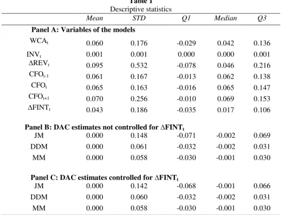
The following table displays the descriptive statistics of the main variables. As shown in expression (6) and discussed above, ∆FINTt seems to be a determinant of WCAt, and both variables tend to have similar distribution as suggested by the values displayed in Table 1-Panel A.
3
If we think that the model is regressed cross-sectionally for a single year but there are firms facing ∆PF and others facing ∆NF the effects are similar to those discussed hereafter.
4
Change in revenues in JM; cash flows from operations of the years t-1, t e t+1 in the DDM; these same cash flows and the change in revenues in MM.
5All statistical analysis is performed using the Statistical Analysis System (SAS) software.
5 Table 1
Descriptive statistics
Mean STD Q1 Median Q3
Panel A: Variables of the models
WCAt 0.060 0.176 -0.029 0.042 0.136
INVt 0.001 0.001 0.000 0.000 0.001
∆REVt 0.095 0.532 -0.078 0.046 0.216
CFOt-1 0.061 0.167 -0.013 0.062 0.138
CFOt 0.065 0.163 -0.016 0.065 0.147
CFOt+1 0.070 0.256 -0.010 0.069 0.153
∆FINTt 0.043 0.186 -0.035 0.017 0.106
Panel B: DAC estimates not controlled for ∆FINTt
JM 0.000 0.148 -0.071 -0.002 0.069
DDM 0.000 0.061 -0.032 -0.002 0.031
MM 0.000 0.058 -0.030 -0.001 0.030
Panel C: DAC estimates controlled for ∆FINTt
JM 0.000 0.142 -0.068 -0.001 0.066
DDM 0.000 0.060 -0.032 -0.002 0.031
MM 0.000 0.058 -0.030 -0.001 0.030
Notes:
Variables definition: WCAt- Working capital accruals in yeart defined as changes in current assets less changes in current liabilities less
changes in cash plus changes in current maturities of long-term debt (See expression (1) ); INVt – is the inverse of average total assets of yeart; ∆REVt – Change in revenue in yeart; CFOt - cash flows from operations in yeart , CFOt-1, CFOt+1 - are the previous and next periods cash flow from operations, respectively; ∆FINTt –Total financing changes in yeart, that includes changes in short-term and long-term bank financing, in loans from shareholders, in equity and in others instruments of equity (e.g., Shan et al., 2010;Zhang, 2007). All variables are deflated by average total assets. The number of observations is 48,041.
By definition of a linear regression, the mean of controlled and not controlled DAC is equal to zero in all models. The values of the remaining distribution moments displayed are very similar for controlled and not controlled estimations. The highlight goes for JM, that shows descriptive statistics twice as high as those of other models.
Table 2 displays correlation coefficients. An emphasis is given to the (expected) positive and statistically significant correlation between WCAtand∆FINTt, and the negative one between ∆FINTtand CFOt.
Table 2
Correlation coefficients Pearson/Spearman
WCAt INVt ∆REVt CFOt CFOt-1 CFOt+1 ∆FINTt Ct
WCAt 1 0.084 0.265 -0.278 0.006## 0.002## 0.263 0.229
INVt 0.093 1 0.210 0.041 0.019 0.051 0.039 0.025
∆REVt 0.316 0.128 1 0.106 -0.054 0.069 0.052 0.031
CFOt -0.271 0.025 0.124 1 -0.038 -0.005## -0.287 -0.258
CFOt-1 -0.002## 0.025 -0.066 0.024 1 0.045 0.002## -0.003##
CFOt+1 0.039 0.036 0.081 0.028 0.133 1 0.005## 0.005##
∆FINTt 0.292 0.055 0.041 -0.353 -0.001## 0.020 1 0.623
Ct 0.249 0.038 0.029 -0.310 -0.002## 0.014 0.851 1
Notes:
6 Moreover, it deserves to be highlighted the small correlation between ∆FINTt and ∆REVt, the only explanatory variables in JM, meaning that ∆REVt tends not to explain the impact of ∆FINTt on WCAt. The correlation between ∆FINTt and CFOt is not also strong, consistent with the above expectation that CFO may not explain the impact of ∆FINTt on WCAt. Thus, the correlation coefficients seem to corroborate the expectation that accruals estimation models whose explanatory variables are weakly correlated with ∆FINTt.
4. RESULTS.
4.1. Accruals models and control for financing changes.
Following the objective for the current study introduced above, three accruals models are used: JM; DDM and MM. As previously explained, each model is regressed in two different versions that differentiate by the control for the sign of ∆FINTt, included in the second version (Ct, a dummy variable that takes value 1 if ∆FINTt>0, 0 otherwise). Table 3 presents the accruals models estimation for each version.
Table 3
Estimated versions of accruals models not controlling (NC)/ controlling (C) for changes in financing
Models JM DDM MM
Exp. Sign NC C NC C NC C
Coef. Coef. Coef. Coef. Coef. Coef.
(P-value) (P-value) (P-value) (P-value) (P-value) (P-value)
Intercept ? 0.048 0.002 0.080 0.041 0.072 0.038
(0.000) (0.108) (0.000) (0.000) (0.000) (0.000)
INVt ? 6.287 5.391
(0.000) (0.000)
∆REVt + 0.086 0.084 0.099 0.096
(0.000) (0.000) (0.000) (0.000)
Ct + 0.079 0.060 0.054
(0.000) (0.000) (0.000)
CFOt-1 ? -0.004 -0.002 0.012 0.014
(0.332) (0.647) (0.005) (0.001)
CFOt - -0.299 -0.252 -0.333 -0.290
(0.000) (0.000) (0.000) (0.000)
CFOt+1 ? 0.001 0.000 -0.014 -0.014
(0.805) (0.941) (0.000) (0.000)
R2 7.12% 11.99% 7.72% 10.38% 16.56% 18.68%
R2 AJUST. 7.12% 11.98% 7.72% 10.37% 16.56% 18.67%
Models:
JMH ST ⟹ VTT ⟹ VT W = ;<+ 41XSYW + 4Z∆[ YW+ QW W = ;<+ 41XSYW + 4Z∆[ YW+ \1TW+ RW]
DDMH ST ⟹ VT W = ;<+ 41T^ W_1 + 4ZT^ W+ 4`T^ Wa1+ QW T ⟹ VT W = ;<+ 41T^ W_1 + 4ZT^ W+ 4`T^ Wa1+ \1TW+RW]
MM H ST ⟹ VTT ⟹ VT W = ;<+ 41T^ W_1 + 4ZT^ W+ 4`T^ Wa1+ 4b∆[ YW+ QW W = ;<+ 41T^ W_1 + 4ZT^ W+ 4`T^ Wa1+ 4b∆[ YW+ \1TW+ RW]
Notes:
Ct - dummy variable that takes the value 1 if ∆FINTt>0, 0 otherwise. The remaining variables defined as per Table 1. JM and MM do not include fixed assets as an independent variable because the dependent variable WCAt does not include the depreciation and amortization component. The number of observations is 48,041.
7 The impact on DAC estimates caused by the inclusion of Ct variable in accruals models is discussed next.
4.2. Graphical analysis.
In section 2 it was anticipated that missing control for ∆FINTt implies that DAC are overestimated for firm-years that recorded ∆PF and underestimated for those recording ∆NF. In order to test these predictions graphical analyses are performed.
For each model, DAC measurement error (ERR) is plotted against the size of the correspondent ∆FINTt, and a dashed line is added to show the ERR average trend.The graphs are easy to read. For example, for JM a ∆FINTt of 20% of total assets (0.2) implies an average ERR of about minus 4% of total assets (-0.03).7
Graph 1
Difference between DACC and DACNC estimates (ERR) by size
7
8 The graphical evidence corroborates the above discussed expectations. DAC do contain a measurement error due to model missing control for ∆FINT. Such an error (ERR = DACC - DACNC) is consistently negative for firm-years reporting ∆PF, meaning that DAC are overestimated; consistently positive for firm-years reporting ∆NF, meaning DAC are underestimated. However, all models reflect in a similar way the impact of changes in corporate financing. The dashed (trend) lines help to assess the similarity across models.
All models, in a similar way, show specification problems related to missing control for financing changes. According to the trend lines we can see that the means of measurement errors are almost similar for small and extreme financing changes. The empirical evidence in the current paper extends, and somehow contradicts, Shan et al. (2010) results, that suggest measurement errors occur mainly for extreme financing changes.
4.3. Simulation analysis.
In this subsection a simulation analysis is performed (e.g., Dechow et al., 1995;Hribar and Collins, 2002;Kothari et al., 2005;Shan et al., 2010). It is a complementary way of testing the quality specification of accruals models, testing whether ERR is statistically different from zero for a given ∆FINT. The aim is to test the robustness of the graphical results discussed above, by computing the probability to commit a Type I error when ERR = 0.
The first step begins by taking the basic sample with 48,041 observations and creates 250 random samples with 1,000 observations. Each sample is extracted from the complete basic sample. This first set of 250 random samples is taken as the simulation set with 0% of contamination, i.e. a set where ERR, the core variable, is assumed to be zero. Based on this set of random samples, the rejection frequencies or Type I error rates are estimated, using a two8 tailed t-test, for confidence levels of 1% and 5%.9
The second step adopts the same procedure described previously with a little difference: the random samples are contaminated with a given percentage of observations that must belong to a particular subset of the basic sample. As observed in the graphical analysis, for all models the trend line shows that the mean of estimation errors are almost similar for small and extreme financing changes. Thus, in order to test whether the results show behaviour similar to that depicted in the graphical analysis, contamination is done using, firstly, observations with extreme positive and negative ∆FINT; secondly, observations with ∆FINT close to zero.10 The contamination process starts with an “infection” rate of 10%, that consists in creating 250 intermediate random samples, without replacement11, of 100 (1,000*10%) observations that belong to the subset of extreme (close to zero) observations; and 250 intermediate random samples, without replacement, of 900 (1,000*(100%-10%)) observations extracted from the whole basic sample. Merging both intermediate samples the output is a set of 250 random samples of 1,000 observations, with a 10% contamination level. The probability of committing Type I errors, and consequently the rejection percentages, can now be estimated as described above.
8
Because the hypothesis (H1) is considered in the alternative way, i.e. that ERR≠0.
9 The average ERR of each of the 250 samples is tested against the null hypothesis (H0) which assumes that the per sample average ERR= 0. The rejection frequencies are
the number of times H0 is rejected, divided by 250.
10 The definition of the subsets of extreme and close to zero observations is as follows. Negative (positive) ∆FINT were split in quartiles. “Extreme observations” are those
below the first quartile (above the third quartile); “close to zero” observations are those that lie above the third quartile (below the first quartile).
9 The results are displayed in Table 4. In Panel A it can be seen that for a contamination level of 0% all DACestimation models seems not well-specified, because they have high rejection rates (0.4% up to 2.0%)12, which are above the level of confidence established (1%). In Panel B, and for the same level of contamination (0%), the rejection percentages increase slightly (8.8% up to 10.4%), which are above the defined level of confidence (5%). Thus, the rejection percentage of H0 is, generically in any of the accruals models, higher than the level of confidence adopted.
12
10 Table 4
Percentages of rejection by degree of contamination
% of contamination 0% 10% 20% 30%
∆FINTt <0 ∆FINTt >0 ∆FINTt <0 ∆FINTt >0 ∆FINTt <0 ∆FINTt >0
< Q 1
>Q3 <Q1 >Q3 <Q
1 >Q3 <Q1 >Q3 <Q
1 >Q3 <Q1 >Q3 Panel A: 1% confidence level
JM 2.0%
50. 0%
80.0 %
44.8
% 51.2%
100. 0%
100.0
% 99.2% 99.2%
100. 0% 100.0 % 100.0 % 100.0 %
DDM 2.0%
80. 4%
84.4 %
60.4
% 43.6%
100. 0%
100.0
% 99.6% 97.2%
100. 0% 100.0 % 100.0 % 100.0 %
MM 0.4%
78. 8%
84.0 %
82.8
% 33.2%
100. 0%
100.0 %
100.0
% 98.4%
100. 0% 100.0 % 100.0 % 100.0 % Panel B: 5% confidence level
JM 8.8%
75. 2%
92.0 %
70.0
% 76.0%
100. 0%
100.0
% 99.6% 99.6%
100. 0% 100.0 % 100.0 % 100.0 % DDM 10.4 % 93. 6% 96.4 % 86.0
% 70.4%
100. 0%
100.0 %
100.0
% 98.8%
100. 0% 100.0 % 100.0 % 100.0 %
MM 9.6%
95. 2%
94.8 %
94.4
% 61.6%
100. 0%
100.0 %
100.0
% 100.0%
100. 0% 100.0 % 100.0 % 100.0 % Notes:
This table displays the percentages of rejection by degree of contamination. The percentages of rejection correspond to the relative number of times, out of 250 tests (t-test) performed, the H0 hypothesis is rejected, i.e., the number of times the ERR average by random sample is statistically different from zero. The mentioned quartiles are defined independently for negative (positive) ∆FINT. For levels of contamination exceeding 40% the percentage of rejection is always 100%.
When the contamination degree increases up to 10% the percentages of rejection increase very significantly for all models, reaching in the case of MM 95.2% for the simulation sample infected with extreme negative financing changes. (∆FINTt<0/<Q1). For DDM and JM the percentages of rejection are similar and higher than the adopted confidence level.
For degrees of contamination up to 20%, for both 1% or 5% levels of confidence, the percentages of rejection goes up to 100%, whatever the nature (“close to zero” or “extreme”) of the measurement errors. The results are in line with graphical analysis discussed above. Thus, it is possible to conclude, once again, that all models studied appear to be not well-specified when do not control for financing changes. There is a measurement error that is statistically different from zero. The percentages of rejection of H0 are, for all models and degrees of contamination, higher than the confidence levels adopted (1% or 5%).
The definition of ∆FINTadopted so far includes financing changes in liabilities and equity. The analysis was replicated considering one at a time changes in liabilities financing, i.e. banks financing, and changes in equity financing. The results were qualitatively similar to those discussed so far. Another robustness test was performed using the level of ∆FINTinstead of dummy variable Ct. Also in this case the results were similar to those discussed.
4.4. Test an existent solution to mitigate the problem.
To demonstrate the existence of measurement errors in discretionary accruals by failure to control the financial changes and to test an existent solution to mitigate this problem for the Portuguese context, we decided to adopt Shan et al. (2010) methodology. Thus, we will try to demonstrate the existence of errors starting with the general discretionary accruals framework introduced by McNichols and Wilson (1988) and used in other studies (e.g., Dechow et al., 2012). Accruals in this framework are partitioned into effective discretionary accruals (DAC*) and effective non-discretionary (NDAC*) components, like this:
TT = Sc T∗+ c T∗ (14)
As DAC* are unobservable, they are generally estimated using one of several alternative empirical models, also used in this study, what implies necessarily the existence of an ERR that reflect the effect of omitted variables in the estimation of DAC*. So estimated
DAC can be written like this:
c T = c T∗+ [[ (15)
11 c T∗=∝ +4e [ + f (16) Or
c T =∝ +4e [ + [[ + f (17)
Because ERR is also unobservable, in practice, the researchers use the following expression with ERR omitted:
c T =∝ +Pe [ + R (18) where
P = 4 + g e [ , [[ ∗ hijj/hkljm (19) P = 4 + n P (20) n P = g e [ , [[ ∗ hijj/hkljm (21)
Thus, the magnitude of the bias depends on the correlation between PART and ERRDg e [ , [[ F,the variance of ERR (hijj and the variance of PART (hkljm .
In addition to the methodology used in this study to estimate the ERR, Shan et al. (2010) used the matched-firm approach based on Kothari et al. (2005).This approaches based on DAC estimation, using also different models of DAC estimation existent in literature, where the sample used is composed by pars of firms matched on financing changes , sector of activity and year. Thus, for each firm of the base sample it exists another one that presents the same financing change, belongs to the same sector of activity and the information is for the same year. The ERR is obtained through the difference of the DAC of each pair of firms.
After performing the matching, according to defined conditions, we obtained two samples with 13,417 observations each, i.e., 26,834 observations in total.
Table 5 shows the bias computed, according to the expression (21), for each DAC model estimation, by quartile, in order to establish a comparison with previous analysis.
Table 5
Bias in testing earnings management
∆FINTt <0 ∆FINTt >0
<Q1 >Q3 <Q1 >Q3
Panel A: DAC with Ct (Dummy from ∆FINT) as an additional regressor
JM 0,052 0,047 -0,034 -0,037
DDM 0,034 0,036 -0,027 -0,023
MM 0,029 0,030 -0,023 -0,019
Panel B: DAC matched on ∆FINT
JM 0,008 0,002 -0,001 -0,016
DDM 0,011 0,008 -0,002 -0,019
MM 0,011 0,005 -0,002 -0,013
According to Table 5 Panel A is possible to see that the bias are, similar to the values of the ERR obtained in the previous section, positives for ∆FINT<0and negatives for ∆FINT>0. In line with those results, the bias, for all models, are almost the same for small and extreme ∆FINT.
Using the matched-firm approach, Panel B, we can see that bias are lower, for all models, to those obtained when we use the initial methodology, i.e., Ct as an additional regressor. They are also negatives for ∆FINT<0 and positives for ∆FINT>0. Further we can observe that bias are lower, for all models, for small or near zero ∆FINT, positives or negatives.
Once confirmed, through other methodology, the existence of DAC estimation errors and bias by the lack of ∆FINT as a dependent variable in DAC estimation models used in literature, we need to assess if some of this methodologies used allow to mitigate, in part or totality, the existence of errors in DAC estimation. Thus, we perform a DAC regression, according to expression (18), for each one of the four (PART) dummy variables in which the sample is divided: PART∆FINT<0/<Q1; PART∆FINT<0/>Q3; PART∆FINT>0/<Q1; and
PART∆FINT>0/<Q3. Table 6 shows the coefficients, of each of the models studied and used methodologies, from PART variable and its
12 Table 6
Regression of DAC on different levels of ∆FINT
∆FINTt <0 ∆FINTt >0
PART∆FINT<0/<Q1 PART∆FINT<0/>Q3 PART∆FINT>0/<Q1 PART∆FINT>0/<Q3
Panel A DAC without control for ∆FINT
JM -0.085 -0.019 -0.003 0.084
(P-value) (0.000) (0.000) (0,109) (0.000)
DDM -0.059 -0.017 -0.005 0.062
(P-value) (0.000) (0.034) (0.023) (0.000)
MM -0.051 -0.013 -0.002 0.050
(P-value) (0.000) (0.000) (0.297) (0.000)
Panel B DAC whit Ct (Dummy of ∆FINT) as additional regressor
JM -0.033 -0.016 -0.037 0.047
(P-value) (0.000) (0.000) (0.000) (0.000)
DDM -0.025 0.019 -0.031 0.040
(P-value) (0.000) (0.000) (0.000) (0.000)
MM -0.022 0.018 -0.025 0.031
(P-value) (0.000) (0.000) (0.000) (0.000)
Panel C DAC matched on ∆FINT
JM -0.083 -0.016 -0.003 0.079
(P-value) (0.000) (0.000) (0.228) (0.000)
DDM -0.055 -0.014 -0.004 0.056
(P-value) (0.000) (0.000) (0.154) (0.000)
MM -0.049 -0.009 -0.002 0.047
(P-value) (0.000) (0.000) (0.430) (0.000)
The realized analysis allows us to formulate the expectation, assuming that firms do not practice earnings management, that in those situations where the effect of ∆FINT is controlled, the coefficient of the variable PART, although different from zero, won´t be statistically significant. However, that isn’t always true, according to the data showed in Table 6. In Panel A and B all coefficients are, generally, different from zero and statistically significant. If for the situation presented in Panel A the results were expected, the same isn’t true relatively to the Panel B, where the Ct variable that controls the ∆FINT is included in models. We can conclude that these results are identical, in what is possible to compare, to those presented by Shan et al. (2010).
In what concerns to data showed in Panel C, we expected coefficients not statistically significant. However, we can see that such situation only occur to PART ∆FINT>0/<Q1 in all models studied. In other situations, all coefficients are statistically significant, which contradicts the results reported by Shan et al. (2010), where the coefficients are all not statistically significant, but only reported for extreme ∆FINT (PART∆FINT<0/<Q1 and PART∆FINT>0/<Q3).
The performed simulation analysis, identical to the one developed by Shan et al.(2010) with DAC as the core variable and not tabulated, reveals that frequencies of rejection, for all percentages of contamination, are higher than the significant levels defined (1% and 5%). This discrepancy is more significant in extreme ∆FINT. To ∆FINT near zero the frequencies of rejection, although higher, are very similar to the significant levels defined. This analyze confirm the results showed in Table 6 Panel C.
The matched-firm approach seems to present evidence that allows mitigating, only to ∆FINT near zero, the errors from discretionary accruals estimation, motivated by the omission of explanatory variables that controls ∆FINT. These results can be explained due to a none statistically significant correlation13 between WCA and PART ∆FINT>0/<Q1 and the type of financing and respective repayment adopted by the firms that operate in a context like the Portuguese one.
For the type of firms that compose the sample used in this study (which are classified as SME and represent the almost totality of firms in Portugal) the financing is done in the short term and hence there are a lot of positives and negatives ∆FINT from short
13 dimension (See Graph 1). On the opposite, in other contexts and with larger firms like those considered by Shan et al.(2010), the financing tends to be for medium and long term and the repayment only occurs by the end of maturity term. Therefore it exists many extreme positives and negatives ∆FINT. According to Dechow et al. (2012) the matching procedure can mitigates misspecification when is applied to a relevant omitted variable in samples with extreme values for that variable, but can exaggerates misspecification in samples with extreme values for another variable.
In summary, we can’t completely solve the problem caused by ∆FINT in discretionary accruals estimation. Thus, we conclude, on the one hand, that it exists an estimation error by the omission in the discretionary accruals estimation models of explanatory variables that controls ∆FINT; on the other hand, that the methodology suggested in the literature to mitigate this problem- the matched-firm approach- isn’t completely effective to the context and discretionary accruals estimation models studied, what is normal according too Dechow et al. (2010) because the measurement error in estimating discretionary accruals is related to industry characteristics and the context where firms operate. Thus, we recommend researchers to realize previous studies to the existence of errors in discretionary accruals estimation and the possibility to mitigate them, mainly in situations where DAC and ∆FINT are central variables in the analysis.
5. SUMMARY.
The aim of the present study was to analyse the specification of accruals models under financing changes. Three of them have been tested empirically: JM, DDM and MM.
Using a methodology based on a comparative static approach, with graphical and simulation analyses, the results supported the expectations: when there are financing changes the accruals models are not well-specified, suffering from an omitted variables bias. Moreover, the analyses showed that the measurement error in accruals estimates depends on the sign of these changes, and occurs regardless of financing changes size.
To mitigate the problemwe tested an existent solution identical to the one that was used by Shan et al.(2010), but such methodology, which use the matched-firm approach on ∆FINT, it is not completely effective to the context and discretionary accruals estimation models studied.
These results are important to researchers that use discretionary accruals in their studies. So, we recommend them to realize previous studies to the existence of errors in discretionary accruals estimation and the possibility to mitigate them, mainly in situations where discretionary accruals and financing changes are central variables in the analysis.
The current study makes three main contributions. Firstly, adding to the available literature, it shows that the measurement error induced by not well-specified accruals models is affected by the sign of financing changes, being different for positive and negative changes. Secondly, it also shows that the estimation errors occur regardless of the size and sign of financing changes.. Thirdly, the results add to the literature on the estimation of accruals in a context of non listed small and medium firms.
14 6. REFERENCES.
Ball, R., and L. Shivakumar, 2006,'The Role of Accruals in Asymmetrically Timely Gain and Loss Recognition'. Journal of
Accounting Research, 44(2), pp. 207-242.
Ball, R., and L. Shivakumar, 2008,'Earnings Quality at Initial Public Offerings'. Journal of Accounting and Economics, 45(2-3), pp. 324-349.
Dechow, P., W. Ge, and C. Schrand, 2010,'Understanding earnings quality: A review of the proxies, their determinants and their consequences'. Journal of Accounting and Economics, 50(2–3), pp. 344-401.
Dechow, P. M., and I. D. Dichev, 2002,'The Quality of Accruals and Earnings: The Role of Accrual Estimation Errors'. Accounting
Review, 77(4), pp. 35.
Dechow, P. M., A. P. Hutton, J. H. Kim, and R. G. Sloan, 2012,'Detecting Earnings Management: A New Approach'. Journal of
Accounting Research, 50(2), pp. 275-334.
Dechow, P. M., S. A. Richardson, and R. G.Sloan, 2008,'The Persistence and Pricing of the Cash Component of Earnings'. Journal of
Accounting Research, 46(3), pp. 537-566.
Dechow, P. M., R. G. Sloan, and A. P. Sweeney, 1995,'Detecting Earnings Management'. Accounting Review, 70(2), pp. 193-225. Gerakos, J., 2012,'Discussion of Detecting Earnings Management: A New Approach'. Journal of Accounting Research, 50(2), pp.
335-347.
Healy, P. M., 1985,'The Effect of Bonus Schemes on Accounting Decisions '. Journal of Accounting & Economics, 26 pp. 75-107. Hribar, P., and D. Collins, 2002,'Errors in Estimating Accruals: Implications for Empirical Research'. Journal of Accounting
Research, 40(1), pp. 105-134.
Johnston, J. 1984, Econometric Methods (McGraw-Hill/ International Editions).
Jones, J. F., 1991,'Earnings Management During Important Relief Investigations'. Journal of Accounting Research, 29(2), pp. 193-228.
Kothari, S. P., A. J. Leone, and C. E. Wasley, 2005,'Performance Matched Discretionary Accrual Measures'. Journal of Accounting
and Economics, 39(1), pp. 163-197.
Liu, M. 2008. Accruals and Managerial Operating Decisions Over the Firm Life Cycle: http://ssrn.com/paper=931523, accessed on August 16, 2010.
Marai, A., and V. Pavlović, 2014,'A Overview of Earnings Management Measurement Approaches: Development and Evaluation'.
FACTA UNIVERSITATIS - Series: Economics and Organization 11(1), pp. 21-36.
McNichols, M., and G. P. Wilson, 1988,'Evidence of Earnings Management from the Provision for Bad Debts'. Journal of Accounting
Research, 26(Supplement), pp. 1-31.
McNichols, M. F., 2002,'Discussion of the Quality of Accruals and Earnings: The Role of Accrual Estimation Errors'. Accounting
Review, 77(4), pp. 61.
Moreira, J. A. 2009. Conditional Conservantism and Accruals Models: Does the Old Problem Remain in the New Models? Porto: Faculdade de Economia da Universidade do Porto.
Peasnell, K. V., P. F. Pope, and S. Young, 2000,'Detecting Earnings Management Using Cross-Sectional Abnormal Accruals Models'.
Accounting & Business Research, 30(4), pp. 313-326.
Richardson, S. A., R. G. Sloan, M. T. Soliman, and I. Tuna, 2005,'Accrual Reliability, Earnings Persistence and Stock Prices'. Journal
of Accounting and Economics, 39(3), pp. 437-485.
Ronen, J., and V. Yaari. 2008, Earnings Management - Emerging Insights in Theory, Practice, and Research (Springer/ New York). Shan, Y., S. L. Taylor, and T. S. Walter. 2010. Errors in Estimating Unexpected Accruals in the Presence of Large Changes in Net
External Financing: http://ssrn.com/paper=1572164, acedido em 11 de setembro de 2010.
Young, S., 1999,'Systematic Measurement Error in the Estimation of Discretionary Accruals: An Evaluation of Alternative Modeling Procedures'. Journal of Business Finance & Accounting, 26(7/8), pp. 833-862.