Repositório ISCTE-IUL
Deposited in Repositório ISCTE-IUL: 2019-05-24
Deposited version: Post-print
Peer-review status of attached file: Peer-reviewed
Citation for published item:
Leão, E. R. & Leão, P. R. (2006). Technological innovations and the interest rate. Journal of Economics (Zeitschrift für Nationalökonomie) . 89 (2), 129-163
Further information on publisher's website: 10.1007/s00712-006-0205-7
Publisher's copyright statement:
This is the peer reviewed version of the following article: Leão, E. R. & Leão, P. R. (2006). Technological innovations and the interest rate. Journal of Economics (Zeitschrift für Nationalökonomie) . 89 (2), 129-163, which has been published in final form at
https://dx.doi.org/10.1007/s00712-006-0205-7. This article may be used for non-commercial purposes in accordance with the Publisher's Terms and Conditions for self-archiving.
Use policy
Creative Commons CC BY 4.0
The full-text may be used and/or reproduced, and given to third parties in any format or medium, without prior permission or charge, for personal research or study, educational, or not-for-profit purposes provided that:
• a full bibliographic reference is made to the original source • a link is made to the metadata record in the Repository • the full-text is not changed in any way
The full-text must not be sold in any format or medium without the formal permission of the copyright holders.
Serviços de Informação e Documentação, Instituto Universitário de Lisboa (ISCTE-IUL) Av. das Forças Armadas, Edifício II, 1649-026 Lisboa Portugal
Phone: +(351) 217 903 024 | e-mail: [email protected] https://repositorio.iscte-iul.pt
The Behaviour of the Nominal Interest Rate in a
World with Technological Innovations
Emanuel Reis Leao∗
October 2000
Abstract
In this paper we look at the behaviour of the nominal interest rate in a world where there are technological innovations that are specific to the banking industry as well as technological innovations in nonbank firms. We find that in a world with technological shocks the nominal interest rate has to adjust so as to make the MPL in banks equal the MPL in nonbank firms. Because the banking sector is very small, the key real variables, including the real wage and the real demand for money, are mainly determined outside the banking industry. Given this behaviour, the nominal interest rate charged by the banks has to adjust so as to make the MPL in banks equal the real wage at the point that corresponds to the amount of hours of work that banks need in order to be able to supply the real amount of credit that is being demanded.
keywords: Dynamic General Equilibrium Models, Inside Money, Cash-in-Advance, Tech-nological Innovations.
JEL Classification Number: E13, E17, E24, E32.
∗Instituto Superior de Ciencias do Trabalho e da Empresa, Avenida das Forças Armadas, 1649-026 Lisboa,
1
Introduction
A key post-war U.S. business cycle fact is the negative correlation between the real interest rate
and real output (King and Watson, 1996). However, in standard RBC models the technological
innovations that drive fluctuations make output and the interest rate move in the same direction.
For instance, a positive technological shock leads not only to an increase in real output but also, by
raising the marginal productivity of capital, to higher interest rates. Since, on the other hand, a
positive shock in technology is propagated into the following periods by the process that generates
the shocks, output also rises in the following periods. As a consequence, RBC models generate
positive correlations between the real interest rate and current and future values of real output
-instead of the negative correlations observed in the U.S. business cycle.
King and Watson show that not only the standard RBC model but also two other benchmark
models, the sticky price model and the liquidity effect model, miss the negative correlation between
the real interest rate and real output.
To address this problem, we add a banking sector to a standard RBC model. The impulse
response experiments we performed with our model show that whereas positive shocks in the
nonbank firms technology make the real interest rate go up, positive shocks in the banks technology
make the real interest rate fall. This implies that, if the technological shocks in banks are strong
enough, stochastic simulations of our model generate negative correlations between the real interest
rate and current and future values of real output - the key post-war business cycle fact difficult to
reproduce in model economies.
This result is particularly relevant because technological innovations over the past few decades
have affected the banking industry with special intensity. In fact, the diffusion of information and
communication technologies (ICT) has been a prime vehicle of technological progress, and services
in general and banking in particular are the main beneficiaries of investment in ICT. For instance,
the category of Financial Institutions - of which banking is the major part - is by now the most
ICT intensive industry in the U.S. as measured by the ratio of computer equipment and software
to value added (Triplet and Bosworth, 2002, Table 2). Section 7.2.2. of the present paper presents
empirical evidence which suggests that technological innovations in banks have been larger than
in the rest of the economy.
The structure of the article is as follows. In section 2, we present the economic environment:
economic flows, preferences, technology, resource constraints and market structure. In section 3,
behaviour is outlined in section 4. In section 5 we write down the market clearing conditions, and
then we show the equations that describe the competitive equilibrium. The calibration of the
model is explained in section 6. Section 7 looks at the impact of technological innovations in bank
and nonbank firms, and then discusses the main results of the paper. The last section makes an
overview and concludes.
2
The Economic Environment
We build a closed economy model with no government. There are H homogeneous households, F
homogeneous firms (nonbank firms) and L homogeneous banks in operation. Firms and banks are
owned by households. As a consequence, both the firms’ and the banks’ profits are distributed
to households (the shareholders) at the end of each period. Only one physical good is produced
(physical output), which can either be consumed or used for investment (i.e., used to increase the
capital stock).
Bank loans are the only source of money to the economy. They are provided in real terms
(i.e. in units of physical output). At the beginning of the period, banks make loans to households
who then use the money to buy consumption goods from the firms. At the end of the period,
households receive the money back from the firms as wage and dividend payments. Afterwards,
households use this money to pay to the banks the principal and interest of the debt contracted
at the beginning of the period. The structure of the model is such that, after all these payments,
households are left with nothing, and must therefore borrow again from the banks at the start of
the new period.
The reason why it seems important to work with this kind of credit structure is the fact that,
in modern economies, most money has its origin in loans from commercial banks to households,
firms or the government (to confirm this we only have to look at the aggregate balance sheet of
the Monetary Sector).
It is important to emphasize that the essence of our extension of the RBC model is not money,
but rather the addition of a banking sector which provides credit and charges interest in real
terms. There is not a nominal money stock, nor a price level. Money is provided in real terms,
and has no effect or function in the economy except that of a means of settling exchanges.
We next examine the typical household’s preferences, the technology available in the economy,
the resource constraints, and the market structure. The typical household seeks to maximize
lifetime utility. Utility in period t is given by u(ct, t), where ct is consumption and tis leisure.
U0= E0 ∙t=∞ P t=0 βtu(ct, t) ¸
, where β is a discount factor (0 < β < 1).
The technology available in this economy is as follows. In each period, the typical firm’s
production function is described by yt= AtF (kt, ndt), where ytis the physical output of the firm,
Atis a technological parameter, ktis the firm’s (pre-determined) capital stock, and ndt is the firm’s
labour demand. The capital accumulation equation of each firm is kt+1= (1 − δ)kt+ it, where it
is investment and δ is the per-period rate of depreciation of the capital stock.
For each bank, there is also a production function that tells how many hours of work the bank
must hire to be able to supply a certain amount of credit in real terms. The technology available
to all banks can be summarized by
bst= Dt(nbt)γ (1)
where bs
t is the bank’s supply of credit in real terms, Dt is a technological parameter, and nbt
is the number of work hours hired by the bank. Also note that we are implicitly assuming that
physical capital in banks is fixed and does not depreciate; and that an improvement in the bank’s
technology can be modelled as an increase in Dt.
The resource constraints in this economy are as follows. Each firm starts period t with a
capital stock, kt, which was determined at the beginning of period (t − 1). Hence, the stock of
capital that enters the production function in period t is pre-determined and cannot be changed
at the beginning or during period t. Each household has an endowment of time per-period which
is normalized to one by an appropriate choice of units. This endowment can be used to work or
to rest. Therefore, we can write ns
t+ t= 1, where nst is the household’s supply of labour during
period t.
Finally, the market structure is as follows. There are five markets: the goods market, the
labour market, the bank loans’ market, the market for firms’ shares and the market for banks’
shares. Labour is homogeneous and perfectly mobile between the two industries of the economy
- the physical output industry and the banking industry. All households, firms and banks are
price-takers. Prices are perfectly flexible and adjust to clear all markets in every period.
3
The Behaviour of Banks and Firms
Banks are profit maximizing firms that make loans to households. The loans imply costs of
bank are given by real interest income minus real wage payments to the bank’s employees:
πbankt = rtbst− wtnbt (2)
where rtis the real interest rate charged for loans, bst is the real amount of credit supplied at
the beginning of period t, and wt is the real wage rate. We assume that banks pay wages and
dividends to households only at the end of each period. Using equation (1), equation (2) becomes
πbankt = rtDt(ntb)γ− wtnbt (3)
Each bank maximizes the Value of its Assets (VA), i.e., the expected discounted value of its
stream of present and future dividends. Therefore, at the beginning of period 0 the typical bank’s
optimization problem is M ax nb t V A = E0 ∙t=∞ P t=0 1 (1+r0)(1+r1)....(1+rt)π bank t ¸
where πbankt is given by (3).
Real profits of each firm in period t are given by sales of output minus the wage bill minus
investment expenditure (all variables in real terms):
πt= AtF (kt, ntd) − wtndt− it (4)
Like banks, firms pay wages and distribute dividends to households at the end of each period.
Each firm maximizes the Value of its Assets (VA). Therefore, at the beginning of period 0 the
typical firm’s optimization problem is
M ax nd t,kt+1 V A = E0 ∙t=∞ P t=0 1 (1+r0)(1+r1)...(1+rt)πt ¸
where πtis given by (4). Note that it= kt+1− (1 − δ)kt. There is also an initial condition for
the capital stock, the standard transversality condition for the capital stock, and non-negativity
constraints.
4
The Typical Household’s Behaviour
To write the typical household’s budget constraint, we have first to understand the way bank loans
and shares work in our model. Bank loans work as follows. At the beginning of period t, each
household borrows from banks bt+1
1+rt units in real terms, and then pays
bt+1
1+rt(1 + rt) = bt+1 units
The shares of firms work as follows. qtf is the real price that someone would have to pay to
buy 100% of firm f at the beginning of period t. zft is the percentage of firm f that the household
bought at the beginning of period (t-1) and sells at the beginning of period t. The shares of banks
work in the same way: qtbank,lis the real price of 100% of bank l at the beginning of period t; and
zbank,lt is the percentage of bank l that the household bought at the beginning of period (t-1) and
sells at the beginning of period t.
In this setting, the typical household’s budget constraint is
wt−1nst−1+ f =FX f =1 zftπft−1+ l=L X l=1 ztbank,lπbank,lt−1 + f =FX f =1 ztfqft + l=L X l=1 ztbank,lqtbank,l+ bt+1 1 + rt = = bt+ ct+ f =FX f =1 zft+1qft + l=L X l=1 zt+1bank,lqtbank,l (5)
The left-hand side of this equation indicates the total amount of money the household obtains
at the beginning of period t - wage earnings, dividend earnings from firms and banks, money
received from selling the shares of firms and banks bought at the beginning of period (t-1), and
the amount of bank loans obtained at the beginning of period t. In turn, the right-hand side
of the equation indicates the amount of money that the household spends at the beginning or
during period t - payment of the debt contracted from the banks at the beginning of period
(t-1), consumption expenditure during period t, and the purchase of shares of firms and banks at
the beginning of period t. Hence, equation 5 simply states that the total amount of money the
household obtains at the beginning of period t must be equal to the amount that the household
spends at the beginning or during period t.
We use the following initial condition to describe the household’s debt position at the beginning
of period 0 b0= w−1ns−1+ f =FX f =1 z0fπf−1+ l=L X l=1 z0bank,lπbank,l−1 (6)
This initial condition states that the household begins period 0 with a debt which equals the
sum of the wage and dividend earnings she receives at the beginning of that period 0 [she receives
these earnings because of the hours she worked during period (−1) and because of the shares of firms and banks she bought at the beginning of period (−1)]. Note that period 0 is not the period where the household’s life starts but rather the period where our analysis of the economy begins
her behaviour). In the appendix, we show that this initial condition arises naturally when we
think back to the initial moment of a closed economy without government and where firms don’t
borrow.
Consequently, at the beginning of period 0, the household is looking into the future and
maximizes U0 = E0 ∙t=∞ P t=0 βtu(ct, t) ¸ subject to (5), (6) and ns
t+ t = 1. The choice variables
are ct, t , nst, bt+1 , zt+1f and z bank,l
t+1 . There are also initial conditions on holdings of shares
[zf0 = H1 and z0bank,l = H1], a standard transversality condition on the pattern of borrowing, and
non-negativity constraints.
5
Market Clearing Conditions and the Competitive Equilibrium
With H homogeneous households, F homogeneous firms and L homogeneous banks, the market
clearing conditions for period 0 are as follows: Hc0+ F i0 = F y0, for the goods market; Hns0 =
F nd
0+ Lnb0, for the labour market; and H1+rb10 = Lb
s
0, for the bank loans market. The market
clearing condition in the shares market is that each firm and each bank should be completely
held by the households. Since households are all alike, each household will hold an equal share of
each firm and of each bank. Therefore, the market clearing conditions in the shares market are
Hz1f = 1 and Hzbank,l1 = 1.
To obtain the system of equations that describes the competitive equilibrium, we put together
in a system the typical household’s first order conditions (which implicitly give the household’s
demand and supply functions), the typical firm’s first order conditions (which give, in an implicit
way, the firm’s demand and supply functions), the typical bank’s first order conditions (which
implicitly give the bank’s demand and supply functions), and the market clearing conditions. We
then assume Rational Expectations and that the production function of each firm is homogeneous
of degree one. After all these steps, and if we define the following new per household variables
kt = HF kt , ndt = FH n d t, nbt = HL n b t, q f t = HF q f t , π f t = HF π f t, q bank,l t = HLq bank,l t and πbank,lt = L Hπ bank,l
t , we can write the system describing the Competitive Equilibrium as
u1(ct, 1 − nst) = λt (7)
u2(ct, 1 − nst) = Et[βλt+1wt] (8)
λt
1 + rt
λtqft = Et h βλt+1 ³ πft + qft+1´i (10) λtqbank,lt = Et h βλt+1 ³
πbank,lt + qbank,lt+1 ´i (11)
bt+1 1 + rt = ct (12) AtF2(kt, ndt) = wt (13) Et£At+1F1¡kt+1, ndt+1 ¢ + (1 − δ)¤= 1 + rt (14) rtDtγ µ L H ¶1−γ¡ nbt¢γ−1= wt (15) ct+ £ kt+1− (1 − δ)kt ¤ = AtF (kt, ndt) (16) nst = ndt + nbt (17) bt+1 1 + rt = µ L H ¶1−γ Dt¡nbt ¢γ (18) zt+1f = 1 H (19) zt+1bank,l= 1 H (20) πft = AtF (kt, ndt) − wtndt− £ kt+1− (1 − δ)kt¤ (21) πbank,lt = rtDt µL H ¶1−γ¡ nbt ¢γ − wtnbt (22) for t = 0, 1, 2, 3, ...
Equations 7-12 have their origin in the typical household’s first order conditions. Equation 12
with the household’s initial debt condition and then using the market clearing conditions from the
shares’ market. In the appendix of Leao (2003), it is explained in detail how this credit-in-advance
constraint appears in period 0 and how, under Rational Expectations, it is propagated into future
periods. Equations 13 and 14 result from the typical firm’s first-order conditions. Equation 15
has its origin in the typical bank’s first-order condition. Equations 16-20 result from the market
clearing conditions. Equation 21 is obtained by multiplying the definition of firm profits by (F/H).
Equation 22 results from multiplying the definition of bank profits by (L/H).
If we consider equation (15) in the context of the whole system, we can understand how this
model binds the real supply of credit (which is given by bs
t = Dt(nbt)γ). As long as the market
determined ratio (wt/rt) is finite, equation (15) determines the variable nbt which through the
banks’ production function determines the supply of credit.
In the simulations below we will use the following firm’s production function and household’s
utility function: AtF (kt, ndt) = At(kt)1−α¡ndt
¢α
and u(ct, t) = ln ct+ φ ln t, respectively.
6
Calibration
In order to study the dynamic properties of the model, we have log-linearized each of the equations
in the system 7-22 around the steady-state values of its variables. The log-linearized system was
then calibrated. To calibrate the log-linearized system we used the following parameters. With
the specific utility function we are using, we obtain
Elasticity of the MU of consumption with respect to consumption -1
Elasticity of the MU of consumption with respect to leisure 0
Elasticity of the MU of leisure with respect to consumption 0
Elasticity of the MU of leisure with respect to leisure -1
where MU denotes “Marginal Utility”. From the U.S. data, we obtain
Investment share of total expenditure in the s.s. (i
y) 0.167 Barro (1993)
Firm workers’ share of the firm’s income (α) 0.58 King et al. (1988)
Labour supply in the steady-state (ns) 0.2 King et al. (1988)
Real interest rate in the steady-state (r) 0.007060 FRED and Barro (1993)
Banks’ share of total “hours of work” in s.s. (HnLnbs) 0.014 BLSD
Bank workers’ share of the bank’s income (γ) 0.271 FDIC
In order to calibrate the steady-state real interest rate, we have computed the average quarterly
Economic Data (FRED) to obtain quarterly values for the Bank Prime Loan Rate for the period
1949-1986 and data from Barro (1993) to obtain quarterly values for the inflation rate in the
same period. To calibrate the Banks’ share of “total hours of work” in the steady-state, we have
computed the average value of the ratio (total hours of work in U.S. commercial banks / total
hours of work in the U.S. economy) for the period 1972:1-1986:12. To do this, we used data from
the web site of the Bureau of Labour Statistics (BLS).1
The parameter γ is equal to the bank workers’ share of the bank’s income. In our model, the
only income banks have is interest income. To calibrate γ we have used the “Historical Statistics
on Banking” from the Federal Deposit Insurance Corporation (FDIC) to compute the average
value of the ratio (commercial banks’ wage payments in the U.S. / commercial banks’ interest
income in the U.S.) for the period 1966-1986. The values for the wage payments of commercial
banks we used were the values for “Employee Salaries & Benefits” which were taken from the table
“Noninterest Income and Noninterest Expense of Insured Commercial Banks” of the FDIC’s web
site2. The values for the commercial banks’ interest income were the values for “Interest Income
on Loans and Leases” which were obtained from the table “Interest Income of Insured Commercial
Banks” in their web site. The values in the preceding tables of the present section imply
Consumption share of total expenditure in the s.s. (HcF y) 0.833
Household’s discount factor (β) 0.993
Per-quarter rate of depreciation of the firm’s capital stock (δ) 0.0047
With these parameter values, the model has steady-state values of physical output,
consump-tion and investment which are 1.4% lower than in a zero growth version of the RBC model
presented in King, Plosser and Rebelo (1988) calibrated with our parameters. This is what we
would expect because in their model transactions occur without the need to use money whereas
in our model households have to borrow from the banks to finance their consumption expenditure
and the supply of credit by the banking industry involves spending some of the resources of the
economy, namely “hours of work”. As a consequence, the amount of “hours of work” left to be
used by the physical output industry is lower (note that the total supply of “work effort” in the
steady-state in this economy is still calibrated as ns = 0.2, i.e., the same value that is used by
King, Plosser and Rebelo).
1The internet address is www.bls.gov 2The internet address is www2.fdic.gov/hsob
7
The Dynamic Properties of the Model
The response of the log-linearized model to shocks in the exogenous variables (At and Dt) can
be obtained using the King, Plosser and Rebelo (1988) method. First, we examine the impact
of shocks in the firms’ technology. Afterwards, we look at the impact of shocks in the banks’
technology. Finally, we study the impact of shocks in both sectors.
7.1
Technological innovations in nonbank firms
In this section, we examine the results of two experiments that use shocks in the firms’ technological
parameter (At): impulse response and stochastic simulation. In order to perform these two
exercises, we assumed that the firms’ technological parameter evolves according to the following
process
ˆ
At= 0.9 ˆAt−1+ εt (23)
where ˆAt denotes the % deviation of At from its steady-state value and εtis a white noise.
7.1.1 Impulse Response
The impulse response experiment we carried out with the model was a 1% shock to the firms’
technological parameter (assuming that there are no shocks to the banks’ technology). This shock
occurs at t = 2. The results are plotted in figures 1 to 8. Several conclusions can be drawn.
First, our model is capable of reproducing the key results that the King, Plosser and Rebelo
(1988) RBC model is able to reproduce. On the one hand, consumption, investment and “hours of
work” are pro-cyclical. On the other hand, consumption is less volatile than output and investment
is more volatile than output. These are very well documented stylized facts about the United States
economy [references on this include Kydland and Prescott (1990) and Backus and Kehoe (1992)].
Note also that the figures for ˆyt, ˆct, ˆıt, ˆnst and ˆwtare very close to the figures we obtain with a
zero growth version of the model in King, Plosser and Rebelo. The reason is that in our model
the banking industry is very small (as can be seen in the values we obtained for the parameters
that calibrate its weight - see Section 6).
Second, the response of consumption is slightly weaker in our model than in the zero growth
version of the King, Plosser and Rebelo model (0.1169% instead of 0.122% deviation from the
consumption in our model is 1.4% lower than in the zero growth version of their model (see end
of Section 6).
Third, work hours in banks and their supply of credit respond positively to the technological
shock (figure 5). The reason is as follows. A positive technological shock implies more physical
output and higher wage and dividend payments in real terms. Knowing these payments (which
will only be made at the end of the period) to be higher, households want to consume more and,
therefore, borrow more. The banking industry responds to this increased demand for credit by
hiring more people in order to be able to supply a higher amount of credit.
Finally, the real interest rate reacts positively to a shock in the firms technology (figure 8).
This result can be explained as follows. When the positive shock to the firms technology occurs,
the marginal product of labour (MPL) increases in firms. Because in equilibrium the value of the
MPL in banks must be equal to the value of the MPL in firms (see equations 13 and 15 above),
the interest rate charged by commercial banks has to increase in order to make the value of the
MPL in banks rise as well. The real interest rate (rt) must necessarily rise because the increase
in nb
t, which is needed to obtain a higher supply of credit in real terms, acts in the direction of
reducing the MPL in banks.
7.1.2 Stochastic Simulation
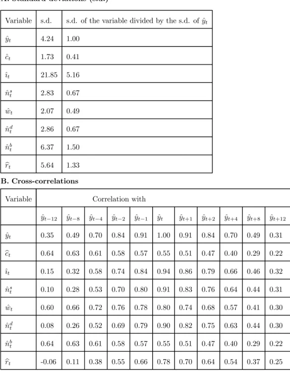
Table 1 shows the results of a stochastic simulation exercise with shocks to the firms’ technological
parameter (with no shocks to the banks’ technological parameter). These results are consistent
with what we obtained in the previous impulse response experiment.
First, the results for the real variables ˆyt, bct, ˆıt, bnst and ˆwt are again very close to the results
we obtained with a zero growth version of the model in King, Plosser and Rebelo (1988).
Second, both ˆnb
tandbrtrespond positively to improvements in the firms technology and,
there-fore, appear positively correlated with output. This stochastic simulation with shocks restricted
to the firm’s technology is thus unable to reproduce the negative correlation between the real
interest rate and real output observed in the U.S. business cycle.
7.2
Technological innovations in both sectors
In this section, we first examine an impulse response experiment that considers shocks only in
the banks’ technological parameter (shocks in Dt), and then we look at what happens when there
are shocks in both sectors (shocks in Atand in Dt). In these experiments, we assumed that the
b
Dt= 0.9 bDt−1+ ϕt (24)
where bDtdenotes the % deviation of Dtfrom its steady-state value and ϕtis a white noise.
7.2.1 Response to a shock in the banks’ technology
Figures 9 to 16 plot the impulse response results of a 1% shock to the banks’ technology (with no
shock in the firms’ technology). It is interesting to see how the economy uses the technological
gift in the banking industry to improve the general welfare of the people that live in it. We
can see that consumption and leisure, the variables that give utility to households, both increase
slightly (figures 10 and 12). This happens because the banking industry now has a more powerful
technology, and can therefore perform its role of supplier of credit using fewer hours of work. Work
hours in banks are reduced by almost 4% (figure 13), and this reduction is used to increase work
hours in firms (figure 14) and to increase leisure (figure 12).
On the other hand, it should be emphasized that the real interest rate falls as a result of the
positive technological shock in the banking sector (figure 16). This can be explained as follows.
The increase in labour demand by firms makes the MPL in firms fall (this can be seen in the fall of
the real wage - figure 15). Since the positive shock in Dt and the ensuing decrease in work hours
in banks both work in the direction of making the MPL rise in banks, the real interest rate must
fall (figure 16) so that the value of the MPL in banks can follow the decrease of the value of the
MPL in firms. This negative impact of the technological innovations in banks on the real interest
rate is the result that made us think it might be possible to replicate the empirical findings of
King and Watson (1996).
7.2.2 Technological innovations bigger in the banking sector
By looking at figures 8 and 16, we can easily see that if a 1% shock in Atis combined with a shock
in Dt which is strong enough, the result will be a fall in the real interest rate. As an example,
figures 17 to 24 plot the impulse response results of a 1% shock in Atcombined with a 5% shock
in Dt. We can see in Figure 24 that the real interest rate falls and in Figure 17 that real output
rises. These impulse response results suggest that negative correlations between the real interest
rate and real output may be obtained in stochastic simulation experiments where the technological
shocks are stronger in banks than in firms.
A question that immediately arises is: does it make sense to use shocks in Dt bigger than
stronger in the banking sector than in the rest of the economy. In fact, and as mentioned in
the introduction to the paper, the banking sector has been the main beneficiary of investment in
ICT - the prime form technological progress has taken in the last few decades. In particular, the
category of Financial Institutions - of which banking is the major part - is by now the most ICT
intensive industry in the U.S. as measured by the ratio of computer equipment and software to
value added (Triplet and Bosworth, 2002, Table 2).
The following facts illustrate the extent to which innovations in the banking industry have
transformed the way it operates. (i) While in the early 1980s the number of ATMs was roughly
equal to the number of bank branches (offices), by 2000 ATMs had outnumbered branches by more
than four to one (Berger, 2003, Table 1). (ii) The ratio between the number of check payments
(which require paper work) and the number of debit and credit card payments (which are almost
entirely processed by electronic means) fell from four in 1995 to only two in 2000 (Gerdes and
Walton, 2002, Table 2). (iii) By the end of 2001, banks with transactional internet websites already
served the majority of bank customers in the U.S. (Furst, Lang and Nolle, 2002).
The effects of these transformations on the productivity statistics have been clear. Productivity
growth has been stronger in the banking sector than in the rest of the economy. According to the
data of the Bureau of Labour Statistics (BLS), between 1982 and 2000 labour productivity grew at
an annual rate of 3.23% in the banking sector against only 1.95% in the private nonfarm business
sector. A study by the Mckinsey Global Institute (2001) estimated an even stronger growth of
labour productivity in the banking sector - an annual rate of 5.36% over the same period.
In our model, technological shocks are measured as percentage deviations from the steady-state
technological trend. In order to obtain an indication about the relative magnitude of the shocks in
Dtand At, we estimated that relationship using real world data. Technological shocks for the total
private sector were estimated as follows. Using the BLS series for the total factor productivity
(TFP) in the private sector - taken from their web site -, we applied the Hodrick-Prescott filter
to estimate the trend, and then calculated the “Percentage deviations from trend of the TFP in
the private sector”.
The estimates for the technological shocks in the banking sector were obtained in the following
way. From the production function of the banking sector (equation 1), we obtained the formula
Dt= b
s t
(nb t)
γ. Values for bst were obtained from the Federal Reserve Economic Data (series “Bank
Credit of Commercial Banks” deflated by the “GDP Implicit Price Deflator” ). Values for nb t
Weekly Hours of Production Workers of Commercial Banks”). For γ, we used the calibration
value (see Section 6). We then used the Hodrick-Prescott filter to estimate the trend of the Dt
series and, finally, computed the “Percentage deviations from trend of the technological levels in
the banking sector”. (We used annual data for the 1980-2000 period).
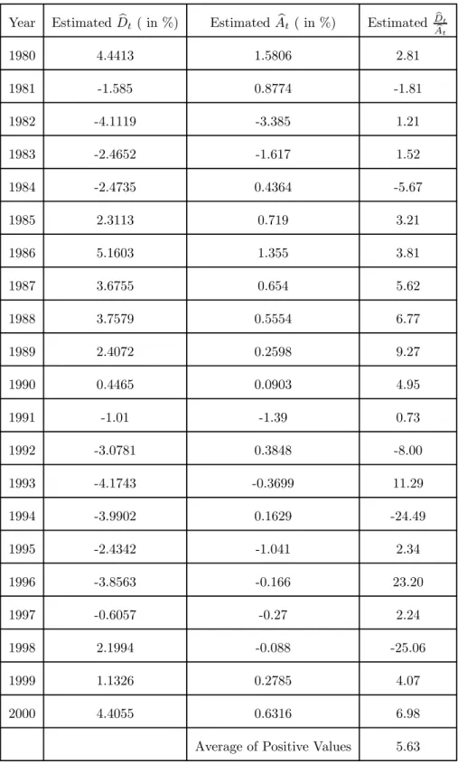
Table 2 shows the estimates for bDtand bAtand the ratio between the two shocks for each year
in the 1980-2000 period. We can see that the shocks in the two sectors were in the same direction
in 16 of the 21 years. In these 16 years, the shocks in the banking industry were on average 5.63
times higher than in the total private sector.
7.2.3 Stochastic simulation with shocks in both sectors
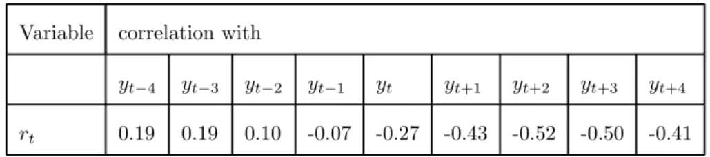
King and Watson (1996) report the following cross-correlations between the real interest rate and
real output in the U.S. data:
Variable correlation with
yt−4 yt−3 yt−2 yt−1 yt yt+1 yt+2 yt+3 yt+4
rt 0.19 0.19 0.10 -0.07 -0.27 -0.43 -0.52 -0.50 -0.41
We can see that, in the real world data, there are negative correlations between the real interest
rate and current and future values of real output.
In our stochastic simulation experiments, we find that if in each period the technological shock
in banks is at least 2.6 times bigger than the technological shock in firms, negative correlations
arise between the real interest rate and current and future real output. Also, if the shock in banks
is 2.8 times larger, the correlation values we obtain are similar to the values reported by King and
Watson.
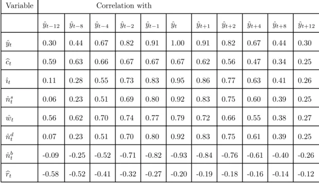
Table 3 shows the results of a stochastic simulation experiment with our model assuming
b
Dt= 2.8 bAt in each period. As shown in Table 3B, this simulation generates correlations between
the real interest rate and current and future values of real output which are not far from the
correlations reported in the King and Watson empirical study. The intuition for this result is
as follows. In our model, a high level of real economic activity comes mainly from the positive
shocks in At. Because each positive shock in Atis propagated into the following periods by the
process which generates the shocks (equation 23), so is a high level of real economic activity
propagated into the following periods. On the other hand, in our simulation each positive shock
in At is associated with a stronger positive shock in Dt which exerts downward pressure on the
real interest rate. As a consequence, negative correlations arise between the real interest rate and
Comparing Tables 1 and 3 we can conclude that the main differences are not only the results
for brtbut also those for ˆnbt. Let us compare the results we report in Table 3B for ˆnbt with the
results for the U.S. data. Using quarterly data for the period 1972-1986 and using a
Hodrick-Prescott filter to estimate the trends, we have obtained a contemporaneous correlation between
“Percentage deviations from trend of work hours in U.S. commercial banks” and “Percentage
deviations from trend of Real GDP in fixed 1992 dollars” equal to −0.158. The data were obtained from the BLS and from the FRED, respectively. While this value does not completely match the
contemporaneous correlation between ˆnb
tand ˆytthat we obtained with our model (which is −0.93
as can be seen in table 3B), it suggests a slightly negative correlation between the two variables
in the U.S. economy. It is obvious from the impulse response exercises and stochastic simulation
exercises we have examined that this negative correlation could only arise in our model if there are
technological innovations in the banking industry. The whole set of correlations we obtain from
the data is
Variable Correlation with
ˆ
yt−12 yˆt−8 yˆt−4 yˆt−2 yˆt−1 yˆt yˆt+1 yˆt+2 yˆt+4 yˆt+8 yˆt+12
ˆ nb
t 0.37 0.53 0.53 0.22 0.07 -0.16 -0.39 -0.59 -0.77 -0.51 -0.013
It may be noted that our results in table 3B also show negative correlations between ˆnbt and
the current and future values of real output. These negative correlations can be explained as
follows. When Atrises, the real income of each household rises which makes them wish to increase
consumption. This causes an increase in the demand for credit in real terms. Since the rise in At
is accompanied by a rise in Dt, the real supply of credit can rise without the need for an increase
in nb t.
We may summarize by saying that the results in Table 3 reproduce the usual results from RBC
models and, at the same time, give us some good results in terms ofbrtand ˆnbt.
8
Conclusion
We have built a dynamic general equilibrium model that adds a banking sector to the standard
RBC model. We have looked at the response of the model to innovations in both the banks’ and
the firms’ technology. In a stochastic simulation exercise with technological shocks that affect
both sectors, but are stronger in the banking sector, we not only reproduce the usual RBC results,
but also obtain interesting results in terms of the cross-correlations between the real interest rate
particularly relevant because the U.S. data show that technological innovations have affected the
banking industry with special intensity.
The main contribution of the paper is to show that technological innovations in banks may
help explain the negative correlation between the real interest rate and current and future values
of real output. This is especially significant because benchmark models have not been able to
reproduce this key feature of the post-war U.S. data.
One avenue for further research is to see if technological shocks in banks can generate similar
References
[1] Backus, D. and Kehoe, P. 1992. International evidence on the historical properties of business
cycles. American Economic Review 82: 864-888.
[2] Barro, R. 1993. Macroeconomics, John Wiley & Sons, Inc.
[3] Berger, A. 2003. The economic effects of technological progress: evidence from the banking
industry. Journal of Money, Credit and Banking 35: 141-176.
[4] Furst, K., Lang, W. and Nolle, D. 2002. Internet banking. Journal of Financial Services
Research 22: 95-117
[5] Gerdes, G. and Walton, J. 2002. The use of checks and other retail non-cash payments in the
United States, Federal Reserve Bulletin, August: 360-374.
[6] King, R., Plosser, C. and Rebelo, S. 1988. Production, growth and business cycles: I. The
basic neoclassical model. Journal of Monetary Economics 21: 195-232.
[7] King, R. and Watson, M. 1996. Money, prices, interest rates and the business cycle. Review
of Economics and Statistics 78: 35-53.
[8] Kydland, F. and Prescott, E. 1990. Business cycles: real facts and a monetary myth. Quarterly
Review. Federal Reserve Bank of Minneapolis, Spring.
[9] Leao, E. 2003. A dynamic general equilibrium model with technological innovations in the
banking sector. Journal of Economics (Zeitschrift für Nationalökonomie) 79: 145-185.
[10] McKinsey Global Institute. 2001. U.S. productivity growth 1995-2000, Washington:
McKin-sey.
[11] Triplet, J. E. and Bosworth, B. P. 2002. Baumol’s disease has been cured: IT and multifactor
APPENDIX
(Not for publication if the article is considered too long; in this case, there would be a note in
the main text saying that this appendix is available on request from the author)
In this appendix we show that the initial condition on the household’s problem that we used
in this paper (equation 6) is the initial condition which naturally arises when we think back to
the initial moment of a closed economy without government and where firms don’t borrow. We
argue that when we start our analysis of the economy at a certain point in time that is in the
middle of History (let us denote this point by period 0), the specific initial condition (describing
the household’s debt position at the beginning of period 0) that we ought to use is the initial
condition we have used in this article.
Let us consider an economy where there are only households, firms and banks and where firms
don’t borrow. Let us imagine that we are at the moment in time where serious economic activity
is going to begin and denote this “Beginning of the economy” period by tB. Since production
is only going to take place during period tB, firms will only receive income from the sales of the
final good during period tB and hence will only pay wages and dividends at the end of period
tB. However, in order to be able to buy consumption goods from the firms during period tB
households must use money. The only possibility they have to obtain this money at the beginning
of period tB is to obtain a loan from a bank. Hence, when the household is at the beginning of
period tB, and considering choices for tB and future periods, she faces the following set of budget
constraints. For period tB the budget constraint is
btB+1 1 + rtB = ctB+ f =FX f =1 qtfB(ztfB+1− zftB) + l=L X l=1
qbank,ltB (ztbank,lB+1 − zbank,ltB ) (25) This budget constraint for period tB simply states that, at the beginning of period tB, the
household must borrow from the banks an amount enough to finance her consumption expenditure
during period tB and to finance her net purchase of shares of firms and of shares of banks.
Since the household is looking into the future, when she is at the beginning of period tB she
also takes into account the budget constraints for periods (tB+ 1), (tB+ 2), (tB+ 3), ... which are
given by wtB−1+in s tB−1+i+ f =FX f =1 zftB+iπftB−1+i+ f =FX f =1 ztfB+iqtfB+i+ l=L X l=1
ztbank,lB+i πbank,ltB−1+i+
l=L
X
l=1
+ btB+1+i 1 + rtB+i = btB+i+ ctB+i+ f =FX f =1 zftB+1+iqtfB+i+ l=L X l=1
zbank,ltB+1+iqtbank,lB+i
for i =1,2,3,...
These budget constraints for periods (tB+1), (tB+2), (tB+3), ... are identical to the household’s
budget constraints examined in section 4 and can be explained in the same way.
Note that when the household is at the beginning of period tB, the budget constraint for tB is
different from the budget constraint for following periods (this happens because at tB there is no
previous period).
In order to derive the initial condition, let us start by writing again equation 25 (the budget
constraint for period tB)
btB+1 1 + rtB = ctB+ f =FX f =1 qtfB(z f tB+1− z f tB) + l=L X l=1 qbank,ltB (z bank,l tB+1 − z bank,l tB )
Imposing here the market clearing conditions in the shares market in period tB (which are
zftB+1=H1 and zbank,ltB+1 = H1) and assuming that the world starts with every household owning the
same share of each firm and each household owning the same share of each bank (so that we also
have ztfB= 1 H and z bank,l tB = 1 H), we obtain btB+1 1 + rtB = ctB (26)
We now write the following tautology
btB+1= btB+1 1 + rtB (1 + rtB) ⇔ btB+1= btB+1 1 + rtB + btB+1 1 + rtB rtB
This tautology simply says that the household’s debt at the end of period tB is equal to the
principal borrowed at the beginning of period tB plus interest on it.
Using equation 26, this last equation becomes
btB+1 = ctB+
btB+1
1 + rtB
rtB
btB+1= F H £ AtBF (ktB, n d tB) − itB ¤ + btB+1 1 + rtB rtB
Using the definition of profits of firm f in period tB (see equation 4), we obtain
btB+1= F H h πftB+ wtBn d tB i + btB+1 1 + rtB rtB ⇔ ⇔ btB+1 = wtB F Hn d tB+ F Hπ f tB+ btB+1 1 + rtB rtB
With the market clearing condition in the labour market (see section 5), this becomes
btB+1= wtB(n s tB− L Hn b tB) + F Hπ f tB+ btB+1 1 + rtB rtB
Using the market clearing condition from the bank loans market (see section 5), we obtain
btB+1= wtB(n s tB− L Hn b tB) + F Hπ f tB+ L Hb s tBrtB Rearranging, we obtain btB+1= wtBn s tB+ F Hπ f tB+ L H £ rtBb s tB− wtBn b tB ¤
Using the definition of nominal profits of bank l in period tB (see equation 2), we obtain
btB+1= wtBn s tB+ F Hπ f tB+ L Hπ bank,l tB
Finally, using the market clearing conditions in the shares market (see section 5), this can be
written as btB+1= wtBn s tB+ f =FX f =1 ztfB+1πftB+ l=L X l=1 zbank,ltB+1 πbank,ltB
Remember that btB+1 denotes the debt that the household has at the beginning of period
(tB+ 1) [ btB +1
1+rtB is the amount borrowed by the household at the beginning of period tB and rtB
is the interest rate between the beginning of period tB and the beginning of period (tB + 1)].
Therefore, this last equation tells us that, in equilibrium, the amount the household borrows at
the sum of the wage earnings and dividend earnings that she will receive there [at the beginning of
period (tB+ 1)]. Hence, when we go on to consider the typical household’s optimization problem
at the beginning of period (tB+ 1) we should add this equation as an initial condition (describing
the debt she carries from the previous period). Therefore, at the beginning of period (tB+ 1) the
household faces the following budget constraints
wtB+in s tB+i+ f =FX f =1 ztfB+1+iπftB+i+ f =FX f =1 zftB+1+iqtfB+1+i+ l=L X l=1
ztbank,lB+1+iπbank,ltB+i +
l=L
X
l=1
zbank,ltB+1+iqtbank,lB+1+i+
+ btB+2+i 1 + rtB+1+i = btB+1+i+ ctB+1+i+ f =FX f =1 zftB+2+iqtfB+1+i+ l=L X l=1
ztbank,lB+2+iqtbank,lB+1+i
for i = 0, 1,2,3,...
plus the initial condition
btB+1= wtBn s tB+ f =FX f =1 ztfB+1πftB+ l=L X l=1 zbank,ltB+1 πbank,ltB
Using the initial condition in the budget constraint written with i =0, the budget constraint
for i = 0 becomes btB+2 1 + rtB+1 = ctB+1+ f =FX f =1 qtfB+1(ztfB+2− ztfB+1) + l=L X l=1
qtbank,lB+1 (ztbank,lB+2 − ztbank,lB+1 )
Therefore the complete description of the budget constraints faced by the household at the
beginning of period (tB+ 1) is btB+2 1 + rtB+1 = ctB+1+ f =FX f =1 qtfB+1(ztfB+2− ztfB+1) + l=L X l=1
qtbank,lB+1 (ztbank,lB+2 − ztbank,lB+1 )
wtB+in s tB+i+ f =FX f =1 ztfB+1+iπftB+i+ f =FX f =1 zftB+1+iqtfB+1+i+ l=L X l=1
ztbank,lB+1+iπbank,ltB+i +
l=L
X
l=1
zbank,ltB+1+iqtbank,lB+1+i+
+ btB+2+i 1 + rtB+1+i = btB+1+i+ ctB+1+i+ f =FX f =1 zftB+2+iqtfB+1+i+ l=L X l=1
ztbank,lB+2+iqtbank,lB+1+i
These two equations are identical in form to the two equations the household was facing at the
beginning of period tB but written one period ahead. Therefore we can repeat the reasoning and
derive an initial condition for the household’s optimization problem at the beginning of period
(tB+ 2). We will obviously obtain a condition which has the same form but written one period
ahead: we obtain btB+2= wtB+1n s tB+1+ f =FX f =1 zftB+2πftB+1+ l=L X l=1 zbank,ltB+2 πbank,ltB+1
(and so on and so forth for all periods ahead). The conclusion to be drawn is that, when we
start our analysis of the economy in the middle of History (in period 0, for example), we should
add to the household’s optimization problem the following initial condition
b0= w−1ns−1+ f =FX f =1 z0fπf−1+ l=L X l=1 z0bank,lπbank,l−1
This is exactly the initial condition we have used in this paper. This initial condition was
derived by thinking back to its initial moment a closed economy without government and where
firms don’t borrow. If instead we think back to its initial moment a closed economy without
government where firms borrow the wages at the beginning of the period (in order to be able
to pay wages in advance at the beginning of the period), the initial condition we obtain is b0 = f =FP
f =1
z0fπf−1 +
l=LP l=1
z0bank,lπbank,l−1 . The results we obtained while working with this other initial
Table 1. Stochastic Simulation. Shocks in the nonbank firms’ technological
para-meter only.
A. Standard deviations (s.d.)
Variable s.d. s.d. of the variable divided by the s.d. of ˆyt
ˆ yt 4.24 1.00 ˆ ct 1.73 0.41 ˆıt 21.85 5.16 ˆ ns t 2.83 0.67 ˆ wt 2.07 0.49 ˆ nd t 2.86 0.67 ˆ nbt 6.37 1.50 brt 5.64 1.33 B. Cross-correlations
Variable Correlation with
ˆ yt−12 yˆt−8 yˆt−4 yˆt−2 yˆt−1 yˆt yˆt+1 yˆt+2 yˆt+4 yˆt+8 yˆt+12 ˆ yt 0.35 0.49 0.70 0.84 0.91 1.00 0.91 0.84 0.70 0.49 0.31 bct 0.64 0.63 0.61 0.58 0.57 0.55 0.51 0.47 0.40 0.29 0.22 ˆıt 0.15 0.32 0.58 0.74 0.84 0.94 0.86 0.79 0.66 0.46 0.32 ˆ ns t 0.10 0.28 0.53 0.70 0.80 0.91 0.83 0.76 0.64 0.44 0.31 ˆ wt 0.60 0.66 0.72 0.76 0.78 0.80 0.74 0.68 0.57 0.41 0.30 ˆ ndt 0.08 0.26 0.52 0.69 0.79 0.90 0.82 0.75 0.63 0.44 0.30 ˆ nb t 0.64 0.63 0.61 0.58 0.57 0.55 0.51 0.47 0.40 0.29 0.22 brt -0.06 0.11 0.38 0.55 0.66 0.78 0.70 0.64 0.54 0.37 0.25
Table 2. Percentage deviations from trend of the technological levels in the banking
sector and in the total private sector, U.S. 1980-2000
Year Estimated bDt( in %) Estimated bAt ( in %) Estimated DAeet
t 1980 4.4413 1.5806 2.81 1981 -1.585 0.8774 -1.81 1982 -4.1119 -3.385 1.21 1983 -2.4652 -1.617 1.52 1984 -2.4735 0.4364 -5.67 1985 2.3113 0.719 3.21 1986 5.1603 1.355 3.81 1987 3.6755 0.654 5.62 1988 3.7579 0.5554 6.77 1989 2.4072 0.2598 9.27 1990 0.4465 0.0903 4.95 1991 -1.01 -1.39 0.73 1992 -3.0781 0.3848 -8.00 1993 -4.1743 -0.3699 11.29 1994 -3.9902 0.1629 -24.49 1995 -2.4342 -1.041 2.34 1996 -3.8563 -0.166 23.20 1997 -0.6057 -0.27 2.24 1998 2.1994 -0.088 -25.06 1999 1.1326 0.2785 4.07 2000 4.4055 0.6316 6.98
Average of Positive Values 5.63
Note: bDtand bAtdenote the percentage deviations from trend of the technological levels in the
banking sector and in the total private sector, respectively.
Table 3. Stochastic simulation. Shocks in the banks’ technology 2.8 times greater
than in the firms’ technology.
A. Standard deviations (s.d.)
Variable s.d. s.d. of the variable divided by the s.d. of ˆyt
ˆ yt 4.26 1.00 ˆ ct 1.78 0.42 ˆıt 20.57 4.83 ˆ ns t 2.66 0.62 ˆ wt 1.91 0.45 ˆ nd t 2.98 0.70 ˆ nb t 20.23 4.75 brt 2.84 0.67 B. Cross-correlations
Variable Correlation with
ˆ yt−12 yˆt−8 yˆt−4 yˆt−2 yˆt−1 yˆt yˆt+1 yˆt+2 yˆt+4 yˆt+8 yˆt+12 ˆ yt 0.30 0.44 0.67 0.82 0.91 1.00 0.91 0.82 0.67 0.44 0.30 bct 0.59 0.63 0.66 0.67 0.67 0.67 0.62 0.56 0.47 0.34 0.25 ˆıt 0.11 0.28 0.55 0.73 0.83 0.95 0.86 0.77 0.63 0.41 0.26 ˆ ns t 0.06 0.23 0.51 0.69 0.80 0.92 0.83 0.75 0.60 0.39 0.25 ˆ wt 0.56 0.62 0.70 0.74 0.77 0.79 0.72 0.66 0.55 0.38 0.27 ˆ nd t 0.07 0.23 0.51 0.70 0.80 0.92 0.83 0.75 0.61 0.39 0.25 ˆ nbt -0.09 -0.25 -0.52 -0.71 -0.82 -0.93 -0.84 -0.76 -0.61 -0.40 -0.26 brt -0.58 -0.52 -0.41 -0.32 -0.27 -0.20 -0.19 -0.18 -0.16 -0.14 -0.12