Asset Allocation
Powered by Information Correlation Flow
Ricardo Emanuel Meneses Casquilho Pereira Supervisor: José Faias
Lisbon, Portugal – 12th of September 2013
Dissertation submitted in partial fulfillment of requirements for the degree of International MSc in Finance, at the Universidade Católica Portuguesa, September 2013
i
Abstract
We propose a new methodology for tactical asset allocation. We allocate by maximizing a power utility function, while switching between the S&P500 and a safe haven asset, the US dollar-euro exchange rate. Also, we use information flows’ correlation as a signal to restrict the opportunity set accordingly. In an out-of-sample exercise, between 1985 and 2013, our signaling methodology is able to yield an annualized Sharpe ratio of 0.91 and an annualized Certainty Equivalent of 17.42%. We are able to the S&P500 which yields an annualized Sharpe Ratio of 0 and annualized Certainty Equivalent of 0.68%.
“They seemed unsure whether the high levels of the stock market might have reflected unjustified optimism, an optimism that might have pervaded our thinking and affected many of our life decisions.”
ii
Acknowledgements
Writing a thesis is always a life-changing event in someone’s life. Comprising of both advances and
regresses, it is as an endless tunnel with emergency lights that one has to go through. Without any of them being the light at the end of the tunnel, one endures and evolves. It is at times like this where
support and companionship are the most important. Thus, I want to thank at everyone who took part in my life during these six months.
I want to thank José Faias, for the outstanding support consistently shown. Thank you as well for being one of the people most liable for the growth I underwent not only due to the thesis but also
due to Empirical Finance. I want to thank Fundação para a Ciência e Tecnologia (FCT) for having assisted me during this last semester. To my friends, I am grateful for your presence. I also want to
express my joy for the time spent with Giulio during these last few years.
Last things first. I want to thank my parents. Undoubtedly, I would have never made it without any
of you. Thank you for being present when most needed. Thank you for the caring and passionate way with which you have created me. Thank you for making me who I am today. Finally, thank you
iii Table of Contents I – Introduction ... 1 II – Data ... 5 III – Methodology ... 6 IV – Empirical Results ... 13
IV.1 – In-Sample Exercise ... 13
IV.2 – Out-of-Sample Exercise ... 15
V – Final Remarks ... 19
iv Index of Tables
Table I – Descriptive statistics for daily observations of S&P500 and $/€ 23
Table II – In-Sample Performance Statistics of IFC Power strategy 24
Table III – Out-of-Sample Performance Statistics of IFC Power strategy between 1985 and 2013 25 Table IV – Out-of-Sample Performance Statistics of IFC Power strategy between 2000 and 2013 26
v
Index of Figures
Figure I – 5-Year Cross-Market Correlation between S&P500 and $/€ 28
Figure II – S&P500 and $/€ realized volatility 29
Figure III – Information Signal 30
1
I – Introduction
“The dollar is regarded as the “safe haven” currency; investors flock to it when they are worried about the outlook for the global economy.”
“The weak shall inherit the Earth” in The Economist – October 6th 2012
Portfolios are often updated, taking into account exogenous signals [Ferson and Siegel (2001), Chambers and Healy (2012)]. Eventually, superior performance is achieved. The used signals
are diverse. There are moving average signals in technical trading [Zhu and Zhou (2009)] and ranking in momentum-based investment strategies [Jegadeesh and Titman (1993)]. Conceptually,
Hansen and Richard (1987) created a new framework for conditional managed portfolios, which has allowed investors to reduce the amount of information they have to pay attention to. A broad strand
of the most diverse dynamic asset allocation models has been derived from it [e.g., among others, Brandt and Santa-Clara (2006), Boissaux and Schiltz (2012)].
We contribute both to the market timing and asset allocation literature. First, we use Fleming, Kirby and Ostdiek (1998) to time the market by investing in S&P500 and the US dollar –
Euro exchange rate. We consider the US dollar as an example of a safe haven asset. By shifting wealth between these two assets, we should be able to enhance the portfolio’s performance. Second,
we create a new framework where the optimal allocation between a risky and a riskless asset is conditioned by the opportunity set. This opportunity set is time-varying and depends on an
exogenous signal.
Dynamic asset allocation depends on investors’ beliefs regarding the future risk-return
tradeoff between different assets. Market timing is one example of a dynamic asset allocation; yet, it has been controversial over time. Some believe that returns are predictable [e.g., Campbell and
2
Thompson (2008), Pastor and Stambaugh (2009)] or that investors – essentially fund managers – have timing ability skills [Larsen Jr and Wozniak (1995), Chen and Liang (2007)]. On the other hand,
there are supporters of both returns not being predictable [e.g., Goyal and Welch (2008)] and the inability of timing markets’ evolution [e.g., Graham and Harvey (1996), Becker et al. (1999)].
In their simplest form, timing portfolios shift the allocation of an investor’s wealth between the market (such as the S&P500) and the risk-free asset, taking into account a given signal [Brandt
and Santa-Clara (2006)]. Mixing equity securities in a portfolio does not always provide the diversification purposes desired during bear markets [Longin and Solnik (2001)]. Optimally, an
investor would like to have safe haven assets in her portfolio so that they would act as a hedge. Investors regard several assets as safe havens: gold [e.g., Baur and McDermott (2010)], currencies
[e.g., Ranaldo and Soderlind (2010), Habib and Stracca (2012)] and others such as bonds or VIX [e.g. Upper (2000), Gulko (2002), Hood and Malik (2013)]. These are regarded as safe haven assets
as they are used during crisis periods, e.g., flight-to-liquidity [Beber, Brandt and Kavajecz (2009)].
Being the US dollar a safe haven, its information flow evolution and its comovement with the S&P500’s could signal market crashes, which in turn may deliver a superior performance.
According to the Bank of International Settlements (BIS), the US dollar is the most liquid currency in the market with roughly 4,652 billion US dollars in global market turnover, followed by the Euro
with about 1,786 US dollar-worth. Also, the US dollar-euro ($/€) exchange rate is the money market leader with about 24% market share.1 Thus, we use $/€ to invest in the US dollar throughout this
dissertation.
3
A safe haven asset – having, on average, negative correlation with equities markets – becomes an expensive hedge if held persistently.2 Thus, it should be held in a timely manner. The
question is whether there is a way that can help us predict financial stress periods to switch towards US dollar, outperforming other asset allocation models. We use an information signal to predict
those periods. Using that signal, we shift between either the S&P500 or the $/€ – depending on the signal provided – while also investing in the risk-free.
Our most innovative feature resides in the signal used: information flow correlation (IFC). We use an information linkage framework so that the performance of traditional asset allocation
models improves. Ross (1989) makes the connection between information and volatility: “in an arbitrage-free economy, the volatility of prices is directly related to the rate of flow of information to
the market”.3 However, it is a cornerstone belief that markets are not fully efficient.4 Taking that into account, we cannot say that volatility is perfectly positively correlated with the rate of flow of
information. Nonetheless, we still assume that there is some degree of positive correlation. We
estimate the IFC between those two assets using Fleming, Kirby and Ostdiek (1998) setup and this is the signal to dynamically change our opportunity set for our asset allocation framework.
How can we connect the information framework to market timing? Stock prices do not frequently reflect their intrinsic value. In fact, the S&P500 is a target of speculative bubbles [e.g.
Shiller (2003)]. Summing up previous findings, the S&P500 usually becomes overvalued until a market crash takes place and its market value adjusts to its fundamentals. Assuming that the
2 There is still no consensus regarding how to distinguish a hedge from a safe haven asset. While some [e.g., Ranaldo and
Soderlind (2010)] assume that hedge and safe haven are the same, i.e. they have, on average, a negative correlation with the market, others [e.g., Baur and Lucey (2010)] consider that a safe haven asset only has a negative correlation with the market during financially stressed periods and positive or no-correlation during other periods.
3 Arbitrage-free economy can be directly connected to market efficiency. While some consider markets to be efficient
[Fama (1970)], wider research defends that they are not fully efficient [e.g. Jegadeesh and Titman (1993) and Shiller (2003)].
4
information flow processes signal investors’ behavior, we invest in the S&P500 whenever the change in IFC is negative and in $/€ whenever the change is positive. We understand from a negative
change that S&P500 is growing beyond reasonable values and by a positive change that the S&P500 is adjusting to its fundamentals.
Driesprong, Jacobson and Maat (2008) find a signaled oil strategy by using the US stock market that yields an annualized Sharpe ratio of 0.72. On a different note, Guidolin and
Timmermann (2008) are able to yield an annualized certainty equivalent of around 10% vs. an annualized average risk-free rate of 5.9% between 1986 and 2005, by investing in equities markets
and using a regime switching model that takes into account bear market’s probability. On our stead, our methodology is able to yield an annualized Sharpe ratio of 0.91 and a Certainty Equivalent of
about 17.42% vs. an annualized average risk-free rate of 9.93%. Regarding safe haven assets and their impact on portfolios, it is surprising to see that there is not much literature about asset
allocation.5 Being negatively correlated with stocks, especially during financial crises, it is only
reasonable that mixing these assets stays at the forefront of the financial research. Ranaldo and Soderlind (2010) show that currencies play the role of a safe haven asset, but not in an asset
allocation framework.
The remaining of this dissertation is organized as follows. Section II explains the data.
Section III explains provides the methodology. Section IV presents the empirical results. Finally, Section V concludes.
5 Also Cenedese (2012) is surprised about how little research there is about safe haven currencies compared to the
5
II – Data
The data consists of daily prices of S&P500 and daily spot prices of the $/€ exchange rate from
1976 to 2013, collected from Bloomberg database. For the $/€ exchange rate, we use the US dollar-Deutsche mark until 1998 and the US dollar-euro from then on, adjusting the return on the change
date. For the risk-free asset, we use daily Ibottson 1-month Treasury-Bill rate collected from Kenneth R. French website.6
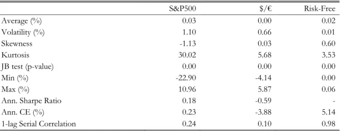
From Table I, the S&P500 yields a larger average return at the expense of being the most
volatile of the risky assets. On its turn, the riskless asset is able to yield a larger average return with a smaller amount of risk. When taking into account risk-adjusted performance metrics, the S&P500
yields a Sharpe ratio of 0.18, lower than its historical value of 0.30. Due to its daily return being on average close to zero, the $/€ presents an extremely negative Sharpe ratio of -0.59. Nevertheless, no
security follows a normal distribution – as they fail to pass the Jarque-Bera test. Therefore, to offset this drawback we also use a power-utility Certainty Equivalent (CE) with a risk parameter of 5. It is
interesting to see that the results remain consistent as the CE is much lower for the $/€ when compared to the S&P500. Even when shorting the $/€, its annualized CE is -1.52%. Still, the
risk-free is able to outperform all other securities by providing a positive annualized CE of 5.14%. Still, the risk-free is an asset with highly persistent returns, while the risky assets have low one-lag serial
correlation.
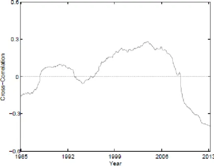
The 5-year cross correlation between S&P500 and $/€ is presented in Figure I. The
correlation is close to zero during most of the sample with three periods of negative correlation. The correlation is negative during the 1987 oil crash and the 2007 financial crisis. Also during the 90s, the
correlation was negative due to the great performance of the S&P500 versus the mediocre evolution
6
of the $/€. For the 2000 financial crash, there is no sharp decrease of the correlation, seeming that the exchange rate did not exhibit a hedge behavior during this period.
Nevertheless, there was a slight stabilization and even a decrease of the exchange rate. Taking these results into account, we expect that a portfolio that uses $/€ as a hedge yields a better
performance during the 1987 and 2007 financial crashes than in the 2000 dotcom bubble burst.
The information flow’s correlation that we use in the signaling of our asset allocation model connects to volatility. We analyze, in Figure II, the evolution of the volatility of S&P500 and $/€.
We present the realized 5-year volatility between 1985 and 2013 for both assets. $/€ volatility is generally lower than the S&P500’s volatility. Thus, the correlation between S&P500 and $/€
volatilities is time-varying. Preceding the 1987 crash, $/€ volatility was decreasing around 1986, when the volatility of S&P500 was still decreasing. Before the 2000 dotcom bubble burst, the
volatility of S&P500 was increasing while the $/€ was decreasing. Also, right before the 2007 financial crisis, $/€ volatility had already stabilized and the S&P500’s was again still decreasing.
Taking this into account, we infer that the correlation of volatilities between the two assets has been decreasing before each financial crisis. So, using as signal a proxy for volatility should enhance the
performance of dynamic allocation models.
III – Methodology
Gladly, investors would collect all possible data when taking their investing decisions. Having limited
time and computational power, investors cannot possibly rank all the different securities [Barber and Odean (2008), Corwin and Coughenour (2008)]. Yet, these are more reasons why decisions might
7
bias [e.g. Coval and Moskowitz (1999)] or a drift to earnings announcements on Friday [Dellavigna and Pollet (2009)]. Investors are not the only ones at fault, since even the media cannot cover all
firms [Fang and Peress (2009)].
As investors cannot be aware of all stocks and in which they should invest, we design an
allocation model, where the opportunity set is restricted to one risky asset out of two possible. One is a proxy for the US stock market, the S&P500, and the other a proxy for a safe haven asset, the US
dollar, through the $/€ exchange rate. In our model, the investor makes her choice using a power utility function:
[ ( )]
(1)
We assume that an investor allocates a total of 100% of his wealth to a portfolio composed of the signaled risky asset and the risk-free. The estimation period is five years. The decision related
to the risk aversion coefficient is never undisputed. Rosenberg and Engle (2002) estimate a risk aversion coefficient between 2.26 and 12.55 using S&P500 option prices. We use a risk aversion
coefficient of 5 [Brandt (2002), Brand and Santa-Clara (2006)].
As the investor holds only one risky and the risk-free asset in her portfolio, the return of the
portfolio is:
( ) ( ) ( ) ( ) (2)
By plugging Equation (2) in Equation (1) and maximizing the investor’s utility, we arrive numerically to the weights resulting from the optimal allocation between the risky and risk-free
8
We provide an information flow-based signal to restrict the opportunity set, only allowing the investor to be long in the risk-free and one security between either S&P500 or $/€. This signal is
computed using a stochastic volatility model which creates a latent information flow process.
In order to compute the information flow correlation – which serves as groundwork for our
asset allocation framework – we have to estimate the volatility asset linkages – or correlation between two volatility processes. While GARCH models have outstanding potential in a univariate
framework, they reveal weaknesses when shifting towards a multivariate framework. They either (1) become much more complex, (2) demand a large number of parameters to be estimated, or (3) lose
some of its tractability. As the subject of this dissertation is related to a multivariate framework, SV models appear as a better alternative to GARCH models. We follow Fleming, Kirby and Ostdiek
(1998) and estimate a bivariate specification, using a GMM model to fit the stochastic volatility processes in the time series of the two risky assets.7
In the context of information, the residual returns usually associated with shocks or
innovations can also be understood as the return yielded by new information. Still, we expect that when there is a greater (smaller) information flow, i.e. there are more (fewer) news arriving, there
exists greater (lower) volatility – from the residual term in Equation (3). We represent such volatility
as , allowing it to follow an AR (1) process – in Equation (4). To create a stochastic volatility
7 An important concern for a risk-averse investor is the degree of risk taken in her positions [Sharpe (1964)]. In a world where uncertainty is present, is of added importance that we try to model and predict such uncertainty. (G)ARCH models [e.g. Engle (1982), Bollerslev (1986)] are one of the most known examples of models. A powerful alternative resides in Stochastic Volatility (SV) models [e.g. Taylor (1982), Hull and White (1987), Harvey, Ruiz and Shephard (1994)], which are known to have a theoretical advantage over GARCH models [e.g. Harvey, Ruiz and Shephard (1994)]. There is also a continuously growing strand of literature that uses Constant Conditional Correlation models [Bollerslev (1990)], Dynamic Conditional Correlations [Engle (2002)] models and Implied Volatility estimated from options [Latane and Rendleman (1976), Harvey and Whaley (1992)]. Nevertheless, apart from the clear interest in estimating volatility more accurately [Jorion (1995), Andersen et al. (2003)], volatility itself has been leveraging several other topics. Just to mention some examples, volatility has been used in the study of the impact of announcements on uncertainty [e.g. Engle and Ng (1993)], risk management [e.g., Engle (2001)] and even option pricing models using not only GARCH models [e.g. Ritchken and Trevor (1999), Barone-Adesi, Engle and Mancini (2008)], but also stochastic volatility [e.g. Hull and White (1987) and Heston (1993)].
9
process [Fleming, Kirby and Ostdiek (1998), Kim, Shephard and Chib (1998)], we use the demeaned log returns of each asset.8 Thus, the daily returns are assumed to follow:
(3)
(4)
However, our aim is to study the impact from the newly arrived information and therefore
we focus on the unpredictable part of the returns: . By linearizing the returns
equation, we are left with:
( ) ( ) (5)
We define:
( ) [ ] (6)
creating as a normalized volatility process, a necessary step before estimating the model
through GMM.9
In our analysis, we use a bivariate GMM model to understand the existence and nature of
volatility linkages. Each stochastic volatility process is fit into each asset’s time series using a mean equation and an AR(1) process:
[ ] [ ] (7)
8 We assume that (
), where is the number of news that arrives to the market for a given asset k on day t [Fleming, Kirby and Ostdiek (1998)]. We adjust such returns for day-of-the-week seasonality and holiday effects. We proceed to further adjustments, if the previous results fail the joint test for serial correlation at a 10% significance level.
10
(8)
(9)
The system of restrictions presented in Equation (10) builds from the moment conditions in
Equations (7), (8) and (9) but in a multivariate framework. As we are dealing with a stochastic
volatility model, we create an unobserved volatility process, , in which we fit . We then create
the first four restrictions of the model as we aim to restrict the first two moments of its distribution for each of the assets. Also, as stated before, we control for volatility persistence, assuming that each
follows an AR(1) process. Thus, we create the fifth and sixth set of restrictions in the model. Then, we control for the correlation of the information linkages between and – seventh
restriction. If markets are to be fully efficient, the two variables are perfectly correlated. Finally, the information flow of one of the assets might have an impact on the persistence term of the second
and for that we create the last two sets of restrictions. We define L, the number of lags in persistence, as 40. Fleming, Kirby and Ostdiek (1998) had already done robustness checks on this
and they discovered that varying L between 10 and 40 would not provide meaningful changes.
( ) ( ( ) ( ) ( ) ( ) ( ) ( ) ( ) ( ) ( ) ( ) ( ) ( ) ( ) ( ) ( ) ( ) ( ) ( ) ( ) ( ) ( ) ) , (10)
11
Here, ( ) is the set of parameters to be
estimated. , and are the mean, variance and persistence parameters of the information
flow process of asset i (mutatis mutandis for asset j). reflects IFC, i.e., the cross-market linkages
between the two risky assets. Finally, reveals the correlation between the disturbance terms of
the stochastic processes of both assets, , where k= i,j from Equation (6), as we aim to control
the possibility that these are correlated. To estimate the parameters of the bivariate specifications we
minimize ( ) ̂ , where ( ) ̅ ( ) and ̂ is a HAC matrix using Parzens weights and
optimal bandwidth selection.10
To estimate the parameters we rebalance on a monthly basis, while using a 5-year rolling
window, starting at December 1985. The estimates using this rolling window are noisier than the ones got through an expanding window. Though, this avoids to progressively decreasing the impact
of new observations, making the signal lethargic as the number of observations accumulate. To prevent cases when the GMM estimation is misspecified, we only take into account estimations
where the p-value of the J-statistic from the model is larger than 10% in order to reduce the uncertainty regarding the soundness of the estimates. In case the model comes misspecified, we take
the estimates from the previous period – and therefore not influencing the allocation.11
For the tactical asset allocation exercise, we use the difference between the IFC and its lagged value as a signal. Yet, how can we interpret this difference as a timing signal using the
S&P500 and $/€? The correlation between S&P500 and $/€ would be greatest if both assets reflected the same information flow: either (1) the S&P500 collapses to its intrinsic value with
investors being extremely concerned with the future outlook or (2) the S&P500 increases according
10 We thank Kostas N. Kyriakoulis for the MatLab GMM toolbox provided. 11 The GMM model J-stat’s p-value is on average 18%.
12
to its fundamentals with investors remaining positive. On the other hand, such correlation would be lowest if (3) the S&P500 had been increasing far beyond its fundamentals with $/€ representing
concerned investors or (4) the S&P500 had been decreasing far past its intrinsic values, while investors remained positive over future prospects. Taking into account what we discussed previously
about S&P500 and $/€, (1) and (3) are more likely to happen. Nevertheless, for asset allocation purposes, what interests us is not the absolute value of such correlation, but its change over time, i.e.
if those relations have been strengthening or weakening through time.
Taking into consideration this reasoning, we assume that an investor allocates her wealth to
the S&P500 whenever there is a decrease in the correlation (negative signal), as the signal warns that it is continuing to grow beyond what fundamentals would advise. Oppositely, whenever it increases
(positive signal), the investor allocates her wealth to a safe haven asset – US dollar in our case – while the S&P500 adjusts to its proper levels. We call this Raw Signaling. One might wonder why we
do not control that investors might be too bearish for what is implicit in the fundamentals or
investment sentiment. The reasons are straightforward: (1) by the inexistence of excessive bullish behavior is considered to be much more likely [Shiller (2003]; (2) intuition tells us that an excessive
bearish behavior should only happen during crisis periods; therefore, its impact on our signal should be mainly decreasing the magnitude of positive signals instead of creating negative signals.
In Figure III, we show the 5-year information flow correlation between S&P500 and $/€ from our stochastic volatility model. After each of the three crises that took place between 1980 and
2013 – 1987 financial crash, 2000 dotcom bubble burst and 2007 financial crisis, – the correlation of the information flow processes of the two chosen assets increases dramatically, following our initial
13
We compare several alternative asset allocation choices through different performance metrics: the first four moments of the distributions, the extremes, annualized Sharpe ratio (SR) and
Certainty Equivalent (CE). The Annualized CE is computed assuming a risk-aversion coefficient equal to the one used in the asset allocation exercise, which is 5. We compare our IFC power model
to four benchmarks: (1) the S&P500, (2) $/€, (3) a naïve portfolio of S&P500 and $/€, and (4) a portfolio that chooses according to a power utility investor. The first two benchmarks are the pure
risky assets; the third assumes that an investor allocates her wealth equally between the two risky and
the risk-free assets. In the fourth, the investor chooses between two risky assets, S&P500 and $/€, and the risk-free by maximizing a power-utility function. Another reason for this choice is that
investors are also concerned about higher moments of the distribution than the mean and variance. For that, we use a power utility function that takes into account all moments of the distribution.
IV – Empirical Results
To understand how well our signal is able to predict markets movements, an asset allocation exercise was performed. Firstly, we analyze the in-sample performance of several asset allocation models.
Secondly, we check the out-of-sample performance. We start by a comparison between the benchmarks, proceed to comparing our model’s performance to the benchmarks’ and conclude by
understanding the role that short-selling takes in the allocation.
IV.1 – In-Sample Exercise
We perform an in-sample exercise that uses a 5-year rolling window estimation period. This is similar to a conditional time-varying in-sample experiment. We averaged all the in-sample
14
presented in Table II. Panel A presents results with no restrictions applied and Panel B assumes no short-selling.
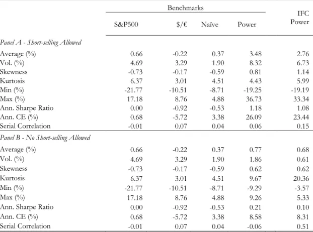
In Panel A, allowing for short selling, a naïve allocation outperforms both the S&P500 and $/€. Even though the return is lower than the S&P500, the small corresponding volatility offsets this
trade-off. Also in a risk-adjusted basis, the naïve yields a better return, both in annualized SR and CE. A power utility investor improves the average performance even further. Even though the risk
is larger, the return is now about ten times larger than the average return of the naïve portfolio. That is noticeable as the annualized SR is 1.18, while the naïve’s is -0.53. The improvement in annualized
CE is remarkable as it is larger by more than 23pp. It is also noteworthy that, with the Power Utility model, the skewness is no longer negative, meaning that there is a larger probability that investors
get positive returns. When applying a signal to restrict the allocation in risky assets to either the S&P500 or $/€ - IFC power portfolio,– the performance still persists. The return is not as large but
the volatility also decreased. Still, the annualized SR is only 9% lower (ann. SR of 1.08) than the
power benchmark portfolio’s. Also the annualized CE is only 3pp lower for the IFC power portfolio, while the skewness is larger.
In Panel B, when short-selling is not allowed, the ranking remains about the same. The power utility portfolios have now lower average return as well as lower volatility. Still, the returns of
both remain around two times the one of the naïve portfolio. This change also decreased the difference in terms of annualized SR for the benchmark power portfolio, which is now 0.21 versus
-0.53 by the naïve portfolio and 0.10 by the IFC power portfolio. The two power utility portfolios yield about the same annualized CE. The difference between their annualized CE and the naïve
15
All in all, the IFC power portfolio yields a far better performance than its benchmarks, apart from the benchmark power portfolio. Such result is reasonable in-Sample as the investor is aware of
the performance of both assets. By restricting the opportunity set we are giving investors less options to go long in assets that have a good performance of short assets that perform badly. Thus,
it is interesting that the gap between the IFC power portfolio and its most direct benchmark is not wider.
IV.2 – Out-of-Sample Exercise
To make a realistic assessment of the effectiveness of the IFC signal, we run an out-of-sample exercise. As stated before, we use a 5-year rolling window to estimate the weights. Also, we
rebalance the positions monthly. The results for the period between 1985 and 2013 are showed in Table III.
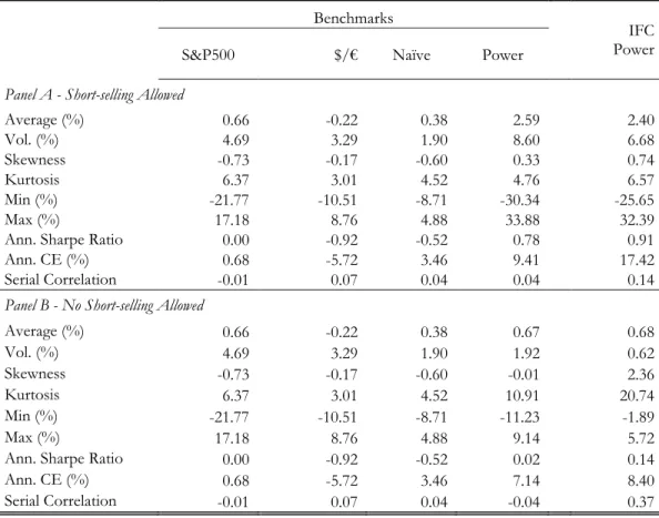
In Panel A, we show the out-of-sample performance when short-selling is allowed. Between the benchmarks, the power utility portfolio remains the best performing model. It is the only model
to yield an average return larger than the average risk-free rate (ann. 9.93%) and therefore the only benchmark with a positive annualized SR. Also in terms of annualized CE, the power utility model
outperforms its peer benchmarks. As expected, the difference is lower than in the in-sample environment but remains at 6pp to the naïve portfolio. Interestingly, the positive skewness
characteristic of this portfolio is still verified. When comparing the benchmark and the IFC power utility portfolios, the ranking has changed. The benchmark only yields a slightly larger return (+7%)
at the expense of being more volatile (+22%) than the IFC portfolio. Still, the annualized SR is about the same. The difference can be perceived through the annualized Certainty Equivalent, which
is 8pp larger for IFC. Also, the model is able to provide investors with a very favorable positive skewness.
16
When not allowing for short-selling, in Panel B, the performance of the power utility portfolios decrease once again. Now, as the average return is lower than the one of the risk-free, also
these yield a negative annualized Sharpe ratio. One should notice that even though this measure is worse for the IFC power portfolio than for the benchmark, such is due to the fact that our return is
able to achieve the same level of return with less than a third of the risk. In fact, one can see that the IFC Power portfolio is the portfolio that yields the highest average return and at the same time the
lowest amount of risk. Such is transferred to the annualized CE as well, being the highest for the
IFC Power portfolio – about 1pp larger than the benchmark power portfolio.
Even though it is optimal to have a large data set to have a better view over the performance of allocation strategies, we also want to see if these strategies have been performing well of lately.
Thus, we show the performance statistics of both the benchmark and IFC portfolios in Table IV, relative to the 2000-2013 period. Also, this period holds a greater importance since it comprises
three financial crises in it.
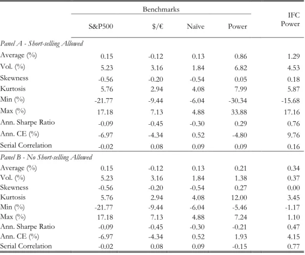
As before, in Panel A, we are able to see the out-of-sample performance of the portfolios when short-selling is allowed. Out of all the benchmarks the power utility portfolio remains the best
in terms of return and annualized Sharpe ratio – the only positive out of all benchmarks. Nevertheless, it exhibits now an annualized Certainty Equivalent of -4.80%, in line with its peers,
being the naïve the best performing benchmark portfolio with 0.52%. During this period, the IFC power portfolio becomes by far the best performing model. Comparing to its most direct
benchmark, it yields a larger return (+50%) and lower volatility (-33%). Consequently, in risk-adjusted metrics, the IFC power more than doubles the Sharpe of the benchmark power portfolio.
Its annualized CE is also 9pp larger than the one of the naïve portfolio, which was the best performing benchmark in this metric. Also noteworthy the fact that allowing for short-selling, the
17
IFC power utility portfolio is able to be less risky than the S&P500 while yielding a return more than ten times as large.
As we do not allow for short positions, in Panel B, the rankings remain the same. The power portfolio is the best performing benchmark: is able to provide the largest average return while being
the less risky. The outcome in terms of Sharpe ratio is not so clear as all are negative, since none was able to surpass the risk-free’s average return (ann. 4.32%). The benchmark power portfolio yields
again the largest annualized Certainty Equivalent of roughly 2%. Nevertheless, it continues to lose to the IFC power portfolio. Ours still yields the largest return at the expense of even less risk than the
benchmark power portfolio. Our methodology is able to outperform the benchmarks also in risk-adjusted terms as it presents a higher annualized Sharpe and CE. Again, our methodology is able to
yield two times the S&P500’s average return while being 93% less volatile.
With a shorter, more recent, period of analysis, the positive-skewness feature has faded. Still, IFC portfolio clearly outperforms all of its benchmarks in whichever performance metric. Our
methodology was able to improve the performance of a simple power utility portfolio by restricting the investors’ opportunity set, according to an information signal.
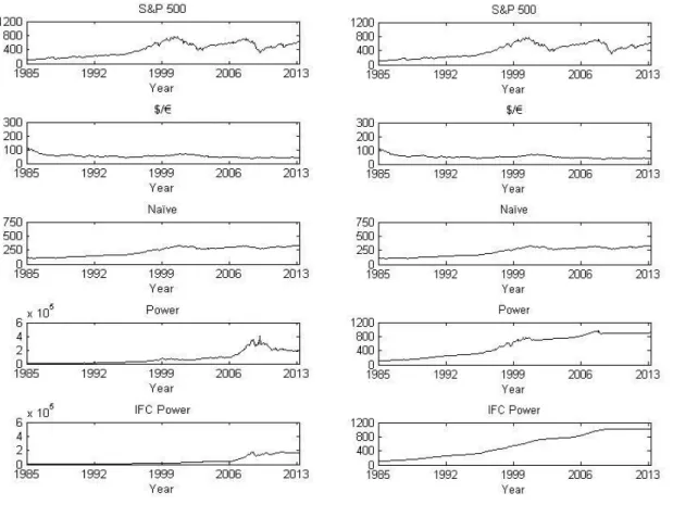
To have a better view over the evolution of the portfolios throughout time, we show Figure IV. In Panel A, we show the cumulative performance of the different portfolios, assuming that
short-selling is allowed. It can clearly be seen a difference in scale between all the different alternatives: an investor invested in the S&P500 would get roughly 14 times the capital she would
get by going long in the $/€. Still, if invested in one of the power portfolios, she would get 223 times the capital she would by going long on the S&P500. The benchmark power portfolio is able to
achieve a maximum cumulative performance unlike any other portfolio. Nevertheless, it eventually drops to values close to the ones of the IFC power portfolio. Having a smoother evolution, it seems
18
reasonable that the IFC has a higher Annualized Certainty Equivalent than the benchmark power portfolio. In Panel B, as we do not allow for short-selling, the cumulative performances of the
power portfolios erode to values close to the ones of the other benchmarks. The power portfolios continue to dominate, with the IFC getting the upper hand. The smoothness and steadiness of its
increase are consistent with the high levels of 1-lag serial correlation reported in Panel B of Tables III and IV.
In Table V, we show the robustness checks regarding Out-of-Sample performance statistics. For robustness checks we run the model to take into account bull and bear markets and then we
change the coefficient of risk-aversion to a level of 2 and 10.
By using the business cycles’ information from the NBER website, we average the returns that belong to either bull or bear markets.12 Having a total number of observations of 342, 308
belong to bull markets, while only 34 stick with bear markets. Taking that into account, the analysis cannot be equally robust in both cases. In Panel A of Table V, we show the Out-of-Sample
performance regarding bull markets. Remaining in the same standings, the power portfolios outperform all others. Still, IFC power is able to attain an annualized SR 13% and an annualized CE
5pp larger than the benchmark power portfolio. When moving to Panel B, we present results for bear markets. The power utility portfolio is able to be the best performing benchmark in terms of
annualized SR (0.45), losing to IFC power’s which is 40% higher. In terms of annualized CE, our model is in line with $/€ and the naïve, the best performing benchmarks.
Moving to Panel C of Table V, we show the returns when the coefficient of risk-aversion is 2. The power portfolio is the best performing benchmark but the IFC Power portfolio stands out as
the one having the best risk-adjusted returns. In terms of annualized SR, it outperforms the power
19
benchmark by 15%, while the annualized CE is larger by 25pp. When changing the same coefficient of risk aversion to 10, our model is still the best, although the difference to the power benchmark
shrinks.
V – Final Remarks
After each financial crisis there is some awakening to the existence of safe haven assets. Most of the
work so far has been to check whether these assets still hold these characteristics. Safe haven assets
only exist because investors recognize in them some inner characteristics that make them feel safe.
We apply an information flows’ correlation methodology created by Fleming, Kirby and Ostdiek (1998) after initial progress by Ross (1989) in an asset allocation framework. By using a
power utility function while restricting the risky assets’ opportunity set between S&P500 and $/€, our methodology greatly improves a standard power utility portfolio performance. In fact, the IFC
power portfolio yields an annualized SR of 0.91 and an annualized CE of 17%, comparing to 0.78
and 9.41% of the benchmark.
We also verify the robustness of our results in terms of business cycles and level of
risk-aversion. We check that our model yields an outstanding annualized CE of 20.62% during bull markets and 31.67% if we change the level of risk-aversion to 2. In fact, our methodology persists as
20
References
Abramowitz, Milton, Stegun, Irene A., 1970, Handbook of Mathematical Functions, Dover Publications, New York.
Andersen, Torben G., Tim Bollerslev, Francis X. Diebold and Paul Labys, 2003, Modeling and Forecasting Realized Volatility, Econometrica 71, 2, 579-625.
Barber, Brad M. and Terrance Odean, 2008, All That Glitters: The Effect of Attention and News on the Buying Behavior of Individual and Institutional Investors, Review of Financial Studies 21, 2, 785-818.
Barone-Adesi, Robert F. Engle and Loriano Mancini, 2008, A GARCH Option Pricing Model with Filtered Historical Simulation, Review of Financial Studies 21, 3, 1223-1258.
Baur, Dirk G. and Brian M. Lucey, 2010, Is gold a hedge or a safe haven? An analysis of stocks, bonds and gold, Financial Review 45, 2, 217-229.
Baur, Dirk G. and T.K. McDermott, 2010, Is gold a safe haven? International evidence, Journal of Banking
and Finance 34, 1886-1898.
Beber, Alessandro, Michael W. Brandt and Kenneth A. Kavajecz, 2009, Quality of Flight-to-Liquidity? Evidence from the Euro-Area Bond Market, Review of Financial Studies 22, 3, 925-957.
Bollerslev, Tim, 1986, Generalized Autoregressive Conditional Heteroskedasticity, Journal of Econometrics 31, 3, 307-327.
Bollerslev, Tim, 1990, Modelling the Coherence in Short-Run Nominal Exchange Rates: A Multivariate Generalized ARCH Model, Review of Economics and Statistics 72, 3, 498-505.
Boissaux, Mark and Jang Schiltz, 2012, Practical weight-constrained conditioned portfolio optimization using risk aversion signals, Luxembourg School of Finance Working Dissertation.
Brandt, Michael W., 2002, Estimating Portfolio and Consumption Choice: A Conditional Euler Equations Approach, Journal of Finance 54, 5, 1609-1645.
Brandt, Michael W. and Pedro Santa-Clara, 2006, Dynamic Portfolio Selection by Augmenting the Asset Space, Journal of Finance 61, 5, 2187-2217.
Campbell, John Y., Karine Serfaty-de-Medeiros and Luis M. Viceira, 2010, Global Currency Hedging,
Journal of Finance 65, 1, 87-121.
Campbell, John Y. and Samuel B. Thompson, 2008, Predicting Excess Stock Returns Out-of-Sample: Can Anything Beat the Historical Average?, Review of Financial Studies 21, 4, 1509-1531.
Cenedese, Gino, 2012, Safe Haven Currencies: A Portfolio Perspective, working dissertation.
Chambers, Christopher P. and Paul J. Healy, 2012, Updating toward the signal, Economic Theory 50, 765-786.
Chen, Yong and Bing Liang, 2007, Do Market Timing Hedge Funds Time the Market?, Journal of Financial
21
Corwin, Shane A. and Jay F. Coughenour, 2008, Limited Attention and the Allocation of Effort in Securities Trading, Journal of Finance 63, 6, 3031-3067.
Coval, Joshua D. and Tobias J. Moskowitz, 1999, Home Bias at Home: Local equity preference in domestic portfolios, Journal of Finance 54, 6, 2045-2073.
Dellavigna, Steffano and Joshua M. Pollet, 2009, Investor Inattention and Friday Earnings Announcements, Journal of Finance 64, 2, 709-749.
Engle, Robert F., 1982, Autoregressive Conditional Hereoscedasticity with Estimates of the Variance of United Kingdom Inflation, Econometrica 50, 4, 987-1007.
Engle, Robert F., 2001, GARCH 101: The Use of ARCH/GARCH Models in Applied Econometrics,
Journal of Economic Perspectives 15, 4, 157-168.
Engle, Robert F., 2002, Dynamic Conditional Correlation: A Simple Class of Multivariate Generalized Autoregressive Conditional Heteroskedasticity Models, Journal of Business & Economics Statistics 20, 3, 339-350.
Engle, Robert F. and Victor K. Ng, 1993, Measuring and Testing the Impact of News on Volatility,
Journal of Finance 48, 5, 1749-1778.
Fama, Eugene F, 1970, Efficient Capital Markets: A Review of Theory and Empirical Work, Journal of
Finance 25, 2, 383-417.
Fang, Lily and Joel Peress, 2009, Media Coverage and the Cross-section of Stock Returns, Journal of
Finance 64, 5, 2023-2052.
Ferson, Wayne E. and Andrew F. Siegel, 2001, The Efficient Use of Conditioning Information in Portfolios, Journal of Finance 56, 3, 967-982.
Fleming, J., C. Kirby and B. Ostdiek, 1998, Information and volatility linkages in the stock, bond and money markets, Journal of Financial Economics 49, 1, 111–37.
Goyal, Amit and Ivo Welch, 2008, A Comprehensive Look at the Empirical Performance of Equity Premium Prediction, Review of Financial Studies 21, 4, 1455-1508.
Graham, John R. and Campbell R. Harvey, 1996, Market Timing Ability and Volatility Implied in Investment Newsletters’ Asset Allocation Recommendations, Journal of Financial Economics 42, 3, 397-421. Gulko, Les, 2002, Decoupling, Journal of Portfolio Management 28, 3, 59-66.
Habib, Maurizio M. and Livio Stracca, 2012, Getting beyond carry trade: What makes a safe haven currency? Journal of International Economics 87, 1, 50-64.
Hansen, Lars Peter and Scott F. Richard, 1987, The Role of Conditioning Information in Deducing Testable Restrictions Implied by Dynamic Asset Pricing Models, Econometrica 55, 3, 587-613.
Harvey, Andrew, Esther Ruiz and Neil Shephard, 1994, Multivariate Stochastic Variance Models, Review of
Economic Studies 61, 2, 247-264.
Harvey, Campbell R. and Robert E. Whaley, 1992, Market volatility prediction and the efficiency of the S&P100 index option market, Journal of Financial Economics 31, 43-73.
22
Heston, Steven L., 1993, A Closed-Form Solution for with Stochastic Volatility with Applications to Bond and Currency Options, Review of Financial Studies 6, 2, 327-343.
Hillier, David, Paul Draper and Robert Faff, 2006, Do Precious Metals Shine? An Investment Perspective, Financial Analysts Journal 62, 2, 98-106.
Hood, Matthew and Farooq Malik, 2013, Is gold the best hedge and a safe haven under changing stock market volatility? Review of Financial Economics 22, 2, 47-52.
Hull, John and Alan White, 1987, The Pricing of Options on Assets with Stochastic Volatilities, Journal of
Finance 42, 2, 281-300.
Jegadeesh, Narasimhan and Sheridan Titman, 1993, Returns to Buying Winners and Selling Losers: Implications for Stock Market Efficiency, Journal of Finance 48, 1, 65-91.
Kim, Sangjoon, Neil Shephard and Siddhartha Chib, 1998, Stochastic Volatility: Likelihood Inference and Comparison with ARCH Models, Review of Economic Studies 65, 3, 361-393.
Larsen Jr., Glen A. and Greggory D. Wozniak, 1995, Market Timing can Work in the Real World: Evidence from a discrete regression model approach, Journal of Portfolio Management 21, 3, 74-81.
Latane, Henry A. and Richard J. Rendleman Jr. Standard deviations of stock price rations implied in option prices, Journal of Finance 31, 2, 369-381.
Longin, François and Bruno Solnik, 2001, Extreme Correlation of International Equity Markets, Journal of
Finance, 56, 2, 649-676.
Pástor, L’Uboš and Robert F. Stambaugh, 2009, Predictive Systems: Living with imperfect Predictors,
Journal of Finance 64, 4, 1583-1628.
Ranaldo, Angelo and Paul Söderlind, 2010, Safe Haven Currencies, Review of Finance 14, 3, 385-407. Ritchken, Peter and Rob Trevor, 1999, Pricing Options under Generalized GARCH and Stochastic Volatility Processes, Journal of Finance 54, 1, 377-402.
Rosenberg, Joshua V. and Robert F. Engle, 2002, Empirical pricing kernels, Journal of Financial Economics 64, 3, 341-372.
Ross, S. A., 1989, Information and Volatility: The No-Arbitrage Martingale Approach to Timing and Resolution Irrelevancy, Journal of Finance 44, 1, 1-17.
Sharpe, William F., 1964, Capital Asset Prices: A Theory of Market Equilibrium under Conditions of Risk, Journal of Finance 19, 3, 425-442.
Shiller, Robert J., 2000, Irrational Exuberance, Princeton University Press.
Shiller, Robert J., 2003, From Efficient Markets Theory to Behavioral Finance, Journal of Economic
Perspectives 17, 1, 83-104.
Taylor, Stephen, 1982, Financial Returns Modelled by the Product of Two Stochastic Processes – a Study of Daily Sugar Prices 1961-79. In Time Series Analysis: Theory and Practice, O.D. Anderson (Ed.), 1, 203-226. Amsterdam: North-Holland.
Zhu, Yingzi and Guogu Zhou, 2009, Technical analysis: An asset allocation perspective over moving averages, Journal of Financial Economics 92, 3, 519-544.
23
Table I – Descriptive statistics for daily observations of S&P500 and $/€
This table presents summary statistics for the S&P500, $/€ exchange rate and the risk-free asset. These statistics are computed with daily data. JB test (p-value) refers to the p-value of the returns Jarque-Bera normality test. The Certainty Equivalent presented assumes a power utility function with a coefficient of risk aversion of 5. 1-lag Serial Correlation is the one-day serial correlation. Values for Sharpe Ratio and Certainty Equivalent are annualized. The number of observations is 9,690.
S&P500 $/€ Risk-Free Average (%) 0.03 0.00 0.02 Volatility (%) 1.10 0.66 0.01 Skewness -1.13 0.03 0.60 Kurtosis 30.02 5.68 3.53 JB test (p-value) 0.00 0.00 0.00 Min (%) -22.90 -4.14 0.00 Max (%) 10.96 5.87 0.06
Ann. Sharpe Ratio 0.18 -0.59 -
Ann. CE (%) 0.23 -3.88 5.14
24
Table II – In-Sample Performance Statistics of IFC Power strategy
This table presents performance statistics (average return, volatility, skewness, kurtosis, minimum, maximum, annualized Sharpe ratio and annualized certainty equivalent) concerning the In-Sample monthly performance of several allocation models. We use daily data from 1980 until 2013. To build these time series, we use a 5-year rolling window used as the estimation period for the Out-of-Sample estimation. In Panel A, we present results that assume short-selling, while in Panel B we do not allow for it. We present four benchmarks: (1) S&P500 and (2) $/€; (3) Naïve, an equally-weighted portfolio of the S&P500, $/€ and risk-free rate and (4) a Power Utility Portfolio, which maximizes the CRRA utility function of an investor – assuming a coefficient of risk aversion of 5. To perform our strategy we take a signal to invest in a risky asset – either in the S&P500 or $/€ – and the risk-free. The signal used in the allocation is the raw change of the correlation of the information flow. To implement the Raw Signaling strategy, we use Power Utility that uses the weight suggested by the power utility portfolio for the signaled risky asset. CE is the power-utility Certainty Equivalent. We assume 5 as the coefficient of risk aversion. The Sharpe Ratio and Certainty Equivalent presented are annualized. The number of estimation periods used is 342.
Benchmarks
IFC Power
S&P500 $/€ Naïve Power
Panel A - Short-selling Allowed
Average (%) 0.66 -0.22 0.37 3.48 2.76 Vol. (%) 4.69 3.29 1.90 8.32 6.73 Skewness -0.73 -0.17 -0.59 0.81 1.14 Kurtosis 6.37 3.01 4.51 4.43 5.99 Min (%) -21.77 -10.51 -8.71 -19.25 -19.19 Max (%) 17.18 8.76 4.88 36.73 33.34
Ann. Sharpe Ratio 0.00 -0.92 -0.53 1.18 1.08
Ann. CE (%) 0.68 -5.72 3.38 26.09 23.44
Serial Correlation -0.01 0.07 0.04 0.06 0.15
Panel B - No Short-selling Allowed
Average (%) 0.66 -0.22 0.37 0.77 0.68 Vol. (%) 4.69 3.29 1.90 1.86 0.61 Skewness -0.73 -0.17 -0.59 0.62 0.62 Kurtosis 6.37 3.01 4.51 9.67 20.36 Min (%) -21.77 -10.51 -8.71 -9.29 -3.57 Max (%) 17.18 8.76 4.88 9.26 5.33
Ann. Sharpe Ratio 0.00 -0.92 -0.53 0.21 0.10
Ann. CE (%) 0.68 -5.72 3.38 8.58 8.31
25
Table III – Out-of-Sample Performance Statistics of IFC Power strategy between 1985 and 2013
This table presents performance statistics (average return, volatility, skewness, kurtosis, minimum, maximum, annualized Sharpe ratio and annualized certainty equivalent) concerning the Out-of-Sample monthly performance of several allocation models. In Panel A, we present results that assume short-selling, while in Panel B we do not allow for it. We present four benchmarks to our strategy: (1) S&P500 and (2) $/€ , (3) Naïve, an equally-weighted portfolio of the S&P500, $/€ and risk-free rate and (4) a Power Utility Portfolio, which maximizes the CRRA utility function of an investor assuming a coefficient of risk aversion of 5. To perform our strategy we take a signal to invest in a risky asset – either in the S&P500 or $/€ – and the risk-free. The signal used in the allocation is the raw change of the correlation of the information flow. To implement the Raw Signaling strategy, we use Power Utility that uses the weight suggested by the power utility portfolio for the signaled risky asset. The weights used are the In-Sample weights from the 5-year estimation period. It is used a 5-year estimation period with monthly rebalancing. CE is the power-utility Certainty Equivalent, assuming 5 as the coefficient of risk aversion. The Sharpe Ratio and Certainty Equivalent presented are annualized. The number of observations is 342.
Benchmarks
IFC Power
S&P500 $/€ Naïve Power
Panel A - Short-selling Allowed
Average (%) 0.66 -0.22 0.38 2.59 2.40 Vol. (%) 4.69 3.29 1.90 8.60 6.68 Skewness -0.73 -0.17 -0.60 0.33 0.74 Kurtosis 6.37 3.01 4.52 4.76 6.57 Min (%) -21.77 -10.51 -8.71 -30.34 -25.65 Max (%) 17.18 8.76 4.88 33.88 32.39
Ann. Sharpe Ratio 0.00 -0.92 -0.52 0.78 0.91
Ann. CE (%) 0.68 -5.72 3.46 9.41 17.42
Serial Correlation -0.01 0.07 0.04 0.04 0.14
Panel B - No Short-selling Allowed
Average (%) 0.66 -0.22 0.38 0.67 0.68 Vol. (%) 4.69 3.29 1.90 1.92 0.62 Skewness -0.73 -0.17 -0.60 -0.01 2.36 Kurtosis 6.37 3.01 4.52 10.91 20.74 Min (%) -21.77 -10.51 -8.71 -11.23 -1.89 Max (%) 17.18 8.76 4.88 9.14 5.72
Ann. Sharpe Ratio 0.00 -0.92 -0.52 0.02 0.14
Ann. CE (%) 0.68 -5.72 3.46 7.14 8.40
26
Table IV – Out-of-Sample Performance Statistics of IFC Power strategy between 2000 and 2013
This table presents performance statistics (average return, volatility, skewness, kurtosis, minimum, maximum, annualized Sharpe ratio and annualized certainty equivalent) concerning the out-of-sample monthly performance of several allocation models. In Panel A, we present results that assume short-selling, while in Panel B we do not allow for it. We present four benchmarks to our strategy: (1) S&P500 and (2) $/€ , (3) Naïve, an equally-weighted portfolio of the S&P500, $/€ and risk-free rate and (4) a Power Utility Portfolio, which maximizes the CRRA utility function of an investor assuming a coefficient of risk aversion of 5. To perform our strategy we take a signal to invest in a risky asset – either in the S&P500 or $/€ – and the risk-free. The signal used in the allocation is the raw change of the correlation of the information flow. To implement the Raw Signaling strategy, we use Power Utility that uses the weight suggested by the power utility portfolio for the signaled risky asset. The weights used are the In-Sample weights from the 5-year estimation period. It is used a 5-year estimation period with monthly rebalancing. CE is the power-utility Certainty Equivalent, assuming 5 as the coefficient of risk aversion. The Sharpe Ratio and Certainty Equivalent presented are annualized. The number of observations is 163.
Benchmarks
IFC Power
S&P500 $/€ Naïve Power
Panel A - Short-selling Allowed
Average (%) 0.15 -0.12 0.13 0.86 1.29 Vol. (%) 5.23 3.16 1.84 6.82 4.53 Skewness -0.56 -0.20 -0.54 0.05 0.18 Kurtosis 5.76 2.94 4.08 7.99 5.87 Min (%) -21.77 -9.44 -6.04 -30.34 -15.68 Max (%) 17.18 7.13 4.88 33.88 17.16
Ann. Sharpe Ratio -0.09 -0.45 -0.30 0.29 0.76
Ann. CE (%) -6.97 -4.34 0.52 -4.80 9.76
Serial Correlation -0.02 0.08 0.09 0.09 0.16
Panel B - No Short-selling Allowed
Average (%) 0.15 -0.12 0.13 0.21 0.34 Vol. (%) 5.23 3.16 1.84 1.38 0.37 Skewness -0.56 -0.20 -0.54 0.27 0.00 Kurtosis 5.76 2.94 4.08 12.00 3.45 Min (%) -21.77 -9.44 -6.04 -5.46 -1.17 Max (%) 17.18 7.13 4.88 7.24 1.10
Ann. Sharpe Ratio -0.09 -0.45 -0.30 -0.21 0.47
Ann. CE (%) -6.97 -4.34 0.52 1.93 4.15
27
Table V – Robustness Checks
This table shows risk-adjusted returns (annualized Sharpe ratio and annualized Certainty Equivalent) regarding robustness checks on the out-of-sample monthly performance of several allocation models. The robustness checks performed concern bull and bear markets (Panel A and B) and changing the level of risk aversion used from 5 to 2 and 10 (Panel C and D).In this table, we t assume short-selling. We present four benchmarks to our strategy: (1) S&P500 and (2) $/€ , (3) Naïve, an equally-weighted portfolio of the S&P500, $/€ and risk-free rate and (4) a Power Utility Portfolio, which maximizes the CRRA utility function of an investor assuming a coefficient of risk aversion of 5. To perform our strategy we take a signal to invest in a risky asset – either in the S&P500 or $/€ – and the risk-free. The signal used in the allocation is the raw change of the correlation of the information flow. To implement the Raw Signaling strategy, we use Power Utility that uses the weight suggested by the power utility portfolio for the signaled risky asset. The weights used are the In-Sample weights from the 5-year estimation period. It is used a 5-5-year estimation period with monthly rebalancing. CE is the power-utility Certainty Equivalent, assuming the same coefficient of risk aversion used in the estimation. The Sharpe Ratio and Certainty Equivalent presented are annualized. The number of observations is 308 for Panel A, 34 for Panel B and 342 for Panels C and
D.
Benchmarks
Power
S&P500 $/€ Naïve Power
Panel A – Bull Markets
Ann. Sharpe Ratio 0.26 -0.95 -0.41 0.87 0.99
Ann. CE (%) 6.53 -5.74 4.58 15.31 20.62
Panel B – Bear Markets
Ann. Sharpe Ratio -1.21 -0.66 -1.19 0.45 0.64
Ann. CE (%) -37.00 -5.54 -5.95 -29.41 -6.95
Panel C - ɣ=2
Ann. Sharpe Ratio 0.00 -0.92 -0.52 0.80 0.92
Ann. CE (%) 5.35 -3.82 4.15 6.14 31.67
Panel D - ɣ=10
Ann. Sharpe Ratio 0.00 -0.92 -0.52 0.76 0.89
28
Figure I – 5-Year Cross-Market Correlation between S&P500 and $/€
The figure shows the contemporaneous correlation between S&P500 and $/€ between 1985 and 2013. To compute the correlation we use a 5-year rolling window.
29
Figure II – S&P500 and $/€ realized volatility
The figure shows, in Panel A, the S&P500 (top) and $/€ (bottom) 5-year realized daily volatilities computed between 1985 and 2013.
30
Figure III – Information Signal
The figure shows the 5-year correlation between the information flow of S&P500 and $/€, using daily data between 1980 and 2013, in a total of 403 observations. It is computed as described in Section III.
31
Figure IV – Cumulative Performance of IFC Power strategy between 1985 and 2013
The figure presents the evolution of the cumulative performance of several allocation models. We present four benchmarks to our strategy: (1) S&P500 and (2) $/€ , (3) Naïve, an equally-weighted portfolio of the S&P500, $/€ and risk-free rate and (4) a Power Utility Portfolio, which maximizes the CRRA utility function of an investor assuming a coefficient of risk aversion of 5. To perform our strategy we take a signal to invest in a risky asset – either in the S&P500 or $/€ – and the risk-free. The signal used in the allocation is the raw change of the correlation of the information flow. To implement the Raw Signaling strategy, we use Power Utility that uses the weight suggested by the power utility portfolio for the signaled risky asset. The weights used are the In-Sample weights from the 5-year estimation period. It is used a 5-year estimation period with monthly rebalancing. In Panel A, we show results assuming that short-selling is allowed, while in Panel B, we assume otherwise. The cumulative performance is shown assuming that the starting base is 100.