CAUSALITY AMONG NEW YORK, LONDON, TOKYO AND HONG KONG STOCK MARKETS

(1)

CAUSALITY AMONG NEW YORK, LONDON, TOKYO AND HONG KONG

STOCK MARKETS

Nissim Ben David Emek Yezreel Academic College

Email: NissimB@yvc.ac.il

ABSTRACT

Investors tend to look into the possibility of broadening their investment activities across countries in order to diversify portfolio risk. This requires an understanding of regional and global linkages of stock markets. In this study, I examine the co-movements in worlds' largest equity markets.I used the daily data of S&P 500, Nikkey 225, Hang Seng and FTSE100 for the period Jan-Nov 2009 in order to examine causality between the markets. Granger causality results show that eastern markets are affected by both S&P 500 and FTSE100, but do not affect western markets. Estimating the rate of change of each index as a function of its lags and of the lags of indexes that were found to granger-cause it, I find a very low predictability for S&P 500, Hang Seng and FTSE100 ,while the Nikkey 225 is pretty highly predictable.

Keywords:causality; predictability; S&P 500; Hang Seng; FTSE100; Nikkey 225

INTRODUCTION

Research for industrialized countries has confirmed that macroeconomic variables influence stock prices (see Mukherjee & Naka (1995), Fifield et al. (2000), Lovatt & Ashok (2000), Nasseh & Strauss (2000), Hondroyiannis & Papapetrou (2001), and Merikas & Merika (2006)). Using annual data covering the years 1960-2000 Kim (2003) found that the S&P 500 stock price is positively related to industrial production, but negatively related to the real exchange rate, interest rate, and inflation. However, the removal of barriers to the free flow of financial capital increased the relationships between equity markets around the world. Fluctuations that occur in one stock market may affect other countries' stock markets, especially in the short run.

The relationships between equity markets in various countries have been extensively examined in previous empirical studies. Arshanapalli, Doukas and Lang (1987) noted an increase in stock market interdependence after the 1987 crisis for the emerging markets of Malaysia, the Philippines, Thailand, and the developed markets of Hong Kong, Singapore, the US and Japan for the period 1986–1992. King and Wadhwani (1990) found that the US market leads other developed markets. Becker et al. (1990) and Hamao et al. (1990) have examined the international linkage between the United States and Japan. They found a high correlation between the two markets with an asymmetric spillover effect from the United States to the Japanese markets. Smith et al. (1993) and Aggerwal and Park (1994), however, found that U.S. equity prices did not lead Japanese equity prices.

Relevant empirical studies have employed a variety of methodologies and have analyzed data from a great number of countries. The identified interdependence was mainly due to the influence which is exerted from the dominant markets. My contribution is to explore the direction of causality across stock markets in 2009 and to examine the predictability of major stock market indexes as a vector auto regression of self and other major stock market indexes.

LITERATURE REVIEW

In the last years, the wide range of technological innovations and internet applications has enabled the instantaneous realization of investors’ decisions from the one side of the planet to the other. As a result, stock exchanges experience higher fluctuations in the price levels and the volume of transactions and their links are made even stronger, enhancing their interdependence. The interdependence among the world stock markets has intensively been studied.

(2)

relationships for six stock market indices and found no lead-lag relationships for the period before and after the market crash, but there were feedback relationships and unidirectional causality during the month of crash.

Narayan et al. (2004) found that stock prices in Bangladesh, India and Sri Lanka Granger-caused stock prices in Pakistan for the period 1995–2001. European countries have also been examined for interdependencies between stock exchange markets. Malliaris and Urrutia (1994) and Gerrits and Yuce (1999) used the concept of Granger causality to analyze the linkage and dynamic interactions among stock prices.

Gklezakou and Mylonakis (2009) examined the relationships among the developing markets of South Eastern Europe before and during the current economic crisis. Their findings suggest that their rather low and vague interdependence has been enhanced.

Mahesh (2005) examined whether there was long-run financial integration between the developed markets of the US, Canada and UK and the emerging markets of India, Malaysia and Singapore. According to his findings, only the pairs Malaysia-Singapore and the US-Canada stock markets exhibited long-run relationships.

Kim (2005) examined the stock market linkages in the advanced Asia-Pacific stock markets of Australia, Japan, Hong Kong and Singapore with the US stock markets. Using the Granger Causality Test on whether the US and Japanese market returns and trading volume Granger caused the market returns of the other markets, he found that the US returns Granger caused returns of each of the stock markets in the region. The Japanese returns, on the other hand, appeared to have a less significant effect.

Rivas et al. (2006) investigated the responses of the stock markets of some Latin American countries, namely, Brazil, Chile and Mexico, to movements in the stock markets in Spain, Italy, Germany, France, UK and the US. The returns of Mexico were significantly influenced by the US market, but returns of Brazil and Chile were affected neither by the US nor the European stock markets.

In this paper, I will examine the causality relations among four major stock markets in 2009 and after detecting the causual direction, I will estimate an adequate Var and will calculate the level of predictability as represented by R2 . The examination will not only give us an idea regarding the causality direction, but will also provide information regarding the possiblility of using previous market information in order to predict future stock martkets returns.

RESEARCH METHODOLOGY Granger Causality Tests

Correlation does not necessarily imply causation in any meaningful sense of the word. The econometric graveyard is full of magnificent correlations, which are simply spurious and/or meaningless. An interesting example includes a positive correlation between teachers' salaries and the consumption of alcohol. The Granger (1969) approach to the question of whether there is causality is to see how much of the current Y can be explained by past values of Y and then to see whether adding lagged values of X can improve the explanation. Y is said to be Granger-caused by X, if X helps in the prediction of Y, or equivalently, if the coefficients on the lagged X's are statistically significant. Since we use time series, we should use only stationary series in order to avoid "spurious" results.

Stationarity

(3)

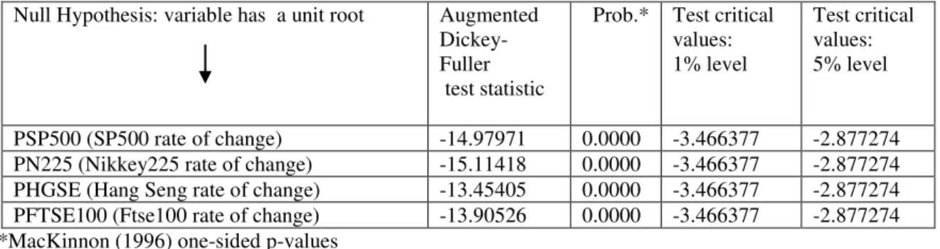
Table 1 Augmented Dickey-Fuller Test Results

Test critical values: 5% level Test critical

values: 1% level Prob.*

Augmented Dickey-Fuller test statistic Null Hypothesis: variable has a unit root

-2.877274 -3.466377

0.0000 -14.97971

PSP500 (SP500 rate of change)

-2.877274 -3.466377

0.0000 -15.11418

PN225 (Nikkey225 rate of change)

-2.877274 -3.466377

0.0000 -13.45405

PHGSE (Hang Seng rate of change)

-2.877274 -3.466377

0.0000 -13.90526

PFTSE100 (Ftse100 rate of change) *MacKinnon (1996) one-sided p-values

Number of Lags in the Var

In general, it is better to use more rather than fewer lags, since the theory is couched in terms of the relevance of all past information. I used two alternatives for the lag length, a granger test with three lags and another test with seven lags. These lag lengths correspond to my reasonable belief about the longest time over which one of the variables could help predict the other.

Table 2 summarizes granger exogeneity test results (see appendix 2, tables 8-9 for detailed results):

Table 2 Granger Exogeneity Test Results

Affected

SP500 HGSE FTSE100 N225

causing

SP500 + + (**) +

HGSE X X +

FTSE100 + (*) + + N225 X X X

(+) column variable causes effected variable (line variable).

(X) column variable does not cause effected variable (line variable).

(*) FTSE100 was found not to be a granger cause of SP500 when using 3 lags, but was found to be a granger cause when using 7 lags.

(**)SP500 was found not to be a granger cause of FTSE100 when using 7 lags, but was found to be a granger cause when using 3 lags.

The results in table 2 show that eastern markets (HGSE and N225) are affected by western markets (S&P 500 and FTSE100) ,but do not affect the western markets, which also effect each other.

The Nikkey 225 is affected by western markets and by the Hang Seng, but does not affect any other market.

It is important to note that the statement "X Granger causes Y" does not imply that Y is the effect or the result of X. Granger causality measures precedence and information content, but does not by itself indicate causality in the more common use of the term.

Vector Auto Regression

(4)

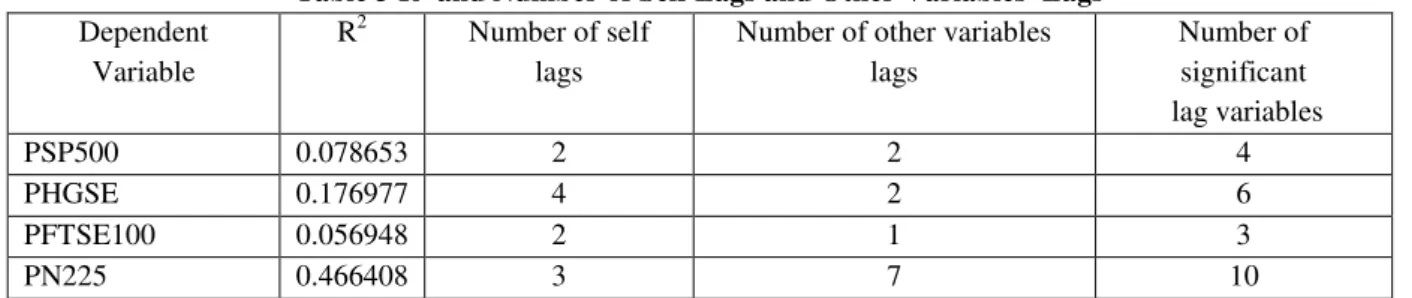
Table 3 R2 and Number of Self Lags and Other Variables' Lags

Dependent Variable

R2 Number of self lags

Number of other variables lags

Number of significant lag variables

PSP500 0.078653 2 2 4

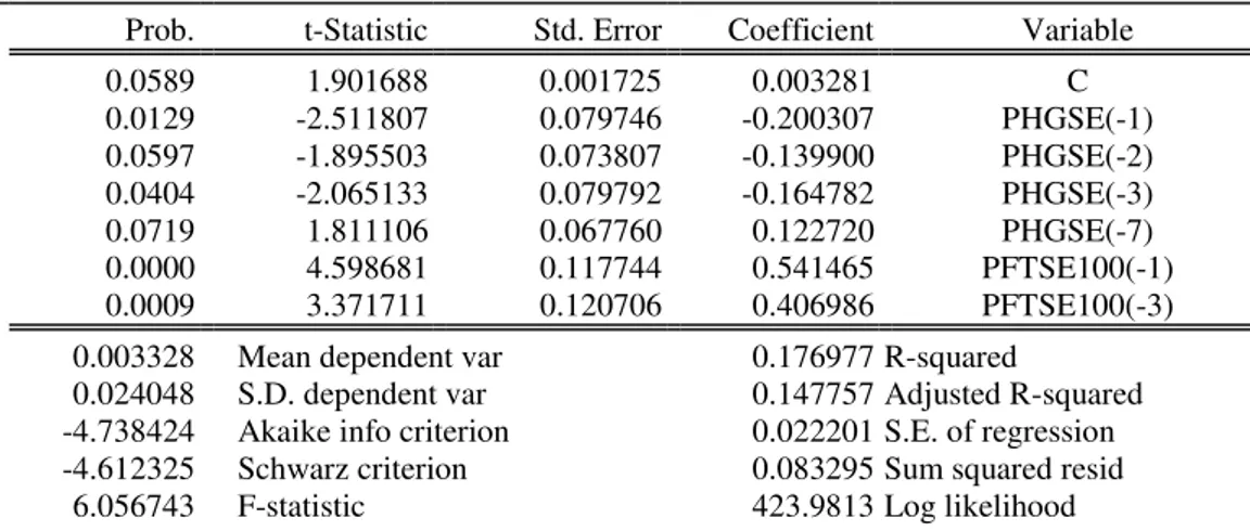
PHGSE 0.176977 4 2 6

PFTSE100 0.056948 2 1 3

PN225 0.466408 3 7 10

As can be seen in table 3, the eastern markets have a higher predictability according to the higher R2 and they are affected by more lag variables in comparison to the western markets. These results are especially true for the Japanese stock market.

SUMMARY

In this paper, I examined causality relations in 2009, according to "Granger" between S&P 500, FTSE, Hang Seng and Nikkei 225. The findings show that eastern markets (Nikkey225 and Hang Seng indexes) are Granger caused by western markets (S&P500 and Ftse100), while western markets affect each other, but are not affected by eastern markets. The Nikkey 225 is affected by all other markets, while it does not affect any other market. The Granger causality test only measures precedence and information content, but does not indicate the predictability of a dependent variable. The fact that S&P "Granger cause" FTSE100 does not mean that past values of S&P 500 returns can determine future FTSE100 returns, but only that past S&P 500 returns contain information that has a certain affect over FTSE100. In order to determine the predictability level, I estimated each of the four indexes as a function of lags of variables that "Granger cause" it. The estimation results show that R2 is very low for S&P 500 and FTSE100 as dependent variables, which means a very low ability to predict future returns, given past returns of variables that granger cause these indexes. For eastern markets, R2 is much higher and is equal to 0.176 for the Hang Seng and 0.47 for the Nikey225 as dependent variables. The R2 is especially high for the Nikey225 which was also found to be "Granger caused" by all other market indexes.

BIBLIOGRAPHY

1. Aggrewal, R. & Park, Y.S. (1994). The relationship between daily U.S. and Japanese equity prices: evidence from spot versus futures markets, Journal of Banking and Finance, 18, 757-773.

2. Arshanapalli, B., Doukas, J. and Lang.L.H.P. (1995). Pre- and post-October 1987 stock market linkages between US and Asian markets, Pacific-Basin Finance Journal, 3, 57–73.

3. Becker, K.G., Finnertly, J.E. and Gupta, M. (1990). The intertemporal relations between the U.S. and Japanese stock markets, Journal of Finance, 45, 1297-1306.

4. Fifield, S., Power, D. and Sinclair. C. (2000). A study of whether macroeconomic factors influence emerging market share returns, Global Economy Quarterly, 1(1), 315-335.

5. Gerrits, R. & Yuce, A. (1999). Short and long term links among European and U.S. stock markets,

Applied Financial Economics, 9, 1-11.

6. Gklezakou, T. & Mylonakis, J. (2009). Interdependence of the developing stock markets, before and during the economic crisis: The case of south Europe, Journal of Money, Investment and Banking, 11, 70-78.

7. Granger, C.W.J. (1969). Investigating Causal Relations by Econometric Methods and Cross-Spectral Methods. Econometrica,34, 424-438.

8. Hamao, Y., Masulis, R.W. and Ng, V. (1990). Correlation in price changes and volatility across international stock markets, Review of Financial Studies, 3, 281-307.

9. Hondroyiannis, G. & Papapetrou, E. (2001). Macroeconomic influences on the stock market, Journal of Economics and Finance, 25(1), 33-49.

(5)

13. Lovatt, D. & Parikh, A. (2000). Stock returns and economic activity: the UK case, European Journal of Finance, 6(3), 280-297.

14. Mahesh, K.T. (2005). A Test of integration between emerging and developed nations' stock markets,

International Finance, Econ WPA.

15. Malliaris, A.G. & Urrutia, J.L. (1992). The International Crash of October 1987: Causality Tests,

Journal of Financial and Quantitative Analysis, 27, 353-364.

16. Merikas, A. G. & Merika, A.A. (2006). Stock prices response to real economic variables: the case of Germany, Managerial Finance, 32 (5), 446-450.

17. Mukherjee, T K. & Naka, A. (1995). Dynamic relations between macroeconomic variables and the Japanese stock market: an application of a vector error correction model, The Journal of Financial Research, 18 (2), 223-237.

18. Najand, M. (1996). A causality test of the October crash of 1987: Evidence from Asian stock markets,

Journal of Business Finance & Accounting, 23, 439–448.

19. Narayan, P., Smyth, R. and Nandha, M. (2004). Interdependence and dynamic linkages between the emerging stock markets of South Asia, Accounting and Finance, 44, 419–439.

20. Nasseh, A. & Strauss, J. (2000). Stock prices and domestic and international macroeconomic activity: A co-integration approach, Quarterly Review of Economics and Finance, 40 (2), 229-245.

21. Rivas, A., Rodriquez, A. and Albuquerque, P.H. (2006). Are European stock markets influencing Latin American stock markets?, Analisis Economico, 21(47), 51-67.

22. Smith, K.L., Brocato, J. and Rogers, J.E. (1993). Regularities in the data between major equity markets: evidence from granger causality tests, Applied Financial Economics, 3, 55-60.

Appendix 1

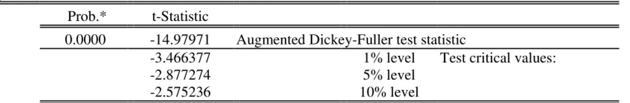
Table 4 Unit root test for S&P 500 Null Hypothesis: PSP500 has a unit root Exogenous: Constant

Lag Length: 0 (Automatic based on SIC, MAXLAG=13)

t-Statistic Prob.*

Augmented Dickey-Fuller test statistic -14.97971

0.0000

Test critical values: 1% level

-3.466377

5% level -2.877274

10% level -2.575236

*MacKinnon (1996) one-sided p-values.

Augmented Dickey-Fuller Test Equation Dependent Variable: D(PSP500) Method: Least Squares

Sample(adjusted): 1/06/2009 9/16/2009

Included observations: 182 after adjusting endpoints

Variable Coefficient

Std. Error t-Statistic

Prob.

PSP500(-1) -1.109532

0.074069 -14.97971

0.0000

C 0.001265

0.001443 0.876412

0.3820

R-squared 0.554887

Mean dependent var -1.82E-05

Adjusted R-squared 0.552414

S.D. dependent var 0.029049

S.E. of regression 0.019434

Akaike info criterion -5.032649

Sum squared resid 0.067983

Schwarz criterion -4.997440

Log likelihood 459.9711

F-statistic 224.3916

Durbin-Watson stat 1.968030

(6)

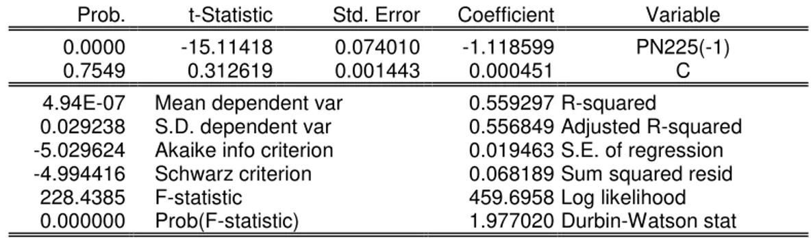
Table 5 Unit root test for PN225

Null Hypothesis: PN225 has a unit root Exogenous: Constant

t-Statistic Prob.*

0.0000

-3.466377

5% level -2.877274

10% level -2.575236

Augmented Dickey-Fuller Test Equation Dependent Variable: D(PN225)

Method: Least Squares

Sample(adjusted): 1/06/2009 9/16/2009

Prob.

PN225(-1) -1.118599

0.074010 -15.11418

0.0000

C 0.000451

0.001443 0.312619

0.7549

R-squared 0.559297

Mean dependent var 4.94E-07

Prob(F-statistic) 0.000000

Table 6 Unit root test for PHGSE Null Hypothesis: PHGSE has a unit root Exogenous: Constant

Lag Length: 0 (Automatic based on SIC, MAXLAG=13) t-Statistic

Prob.*

0.0000

-3.466377

5% level -2.877274

10% level -2.575236

Augmented Dickey-Fuller Test Equation Dependent Variable: D(PHGSE) Method: Least Squares

Sample(adjusted): 1/06/2009 9/16/2009

Prob.

PHKSE(-1) -1.002817

0.074536 -13.45405

0.0000

C 0.002374

0.001826 1.300017

0.1953

R-squared 0.501401

(7)

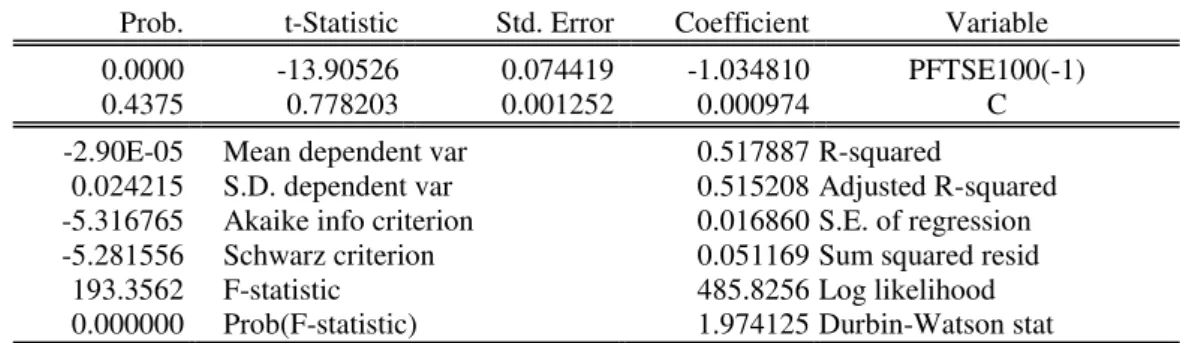
Table 7 Unit root test for PFTSE100 Null Hypothesis: PFTSE100 has a unit root Exogenous: Constant

t-Statistic Prob.*

0.0000

-3.466377

5% level -2.877274

10% level -2.575236

Augmented Dickey-Fuller Test Equation Dependent Variable: D(PFTSE100) Method: Least Squares

Sample(adjusted): 1/06/2009 9/16/2009

Prob.

PFTSE100(-1) -1.034810

0.074419 -13.90526

0.0000

C 0.000974

0.001252 0.778203

0.4375

R-squared 0.517887

Mean dependent var -2.90E-05

Appendix 2

Table 8 Granger exogeneity test with 3 lags Pairwise Granger Causality Tests

Sample: 1/05/2009 11/25/2009 Lags: 3

Null Hypothesis: Obs

F-Statistic Probability

PSP500 does not Granger Cause PN225 180

37.9059 0.00000

PN225 does not Granger Cause PSP500 0.45778

0.71215

PHGSE does not Granger Cause PN225 180

3.57591 0.01519

PN225 does not Granger Cause PHGSE 0.79829

0.49638

PFTSE100 does not Granger Cause PN225 180

23.8859 5.5E-13

PN225 does not Granger Cause PFTSE100 1.53755

0.20654

PHGSE does not Granger Cause PSP500 180

1.05423 0.37008

PSP500 does not Granger Cause PHGSE 26.0162

6.1E-14

PFTSE100 does not Granger Cause PSP500 180

2.02483 0.11222

PSP500 does not Granger Cause PFTSE100 2.52326

0.05938

PFTSE100 does not Granger Cause PHGSE 180

12.4578 2.0E-07

PHGSE does not Granger Cause PFTSE100 0.67063

(8)

Table 9 Granger exogeneity test with 7 lags Pairwise Granger Causality Tests

Sample: 1/05/2009 11/25/2009 Lags: 7

Null Hypothesis: Obs

F-Statistic Probability

PSP500 does not Granger Cause PN225 176

15.4690 2.1E-15

PN225 does not Granger Cause PSP500 0.91293

0.49801

PHGSE does not Granger Cause PN225 176

2.34985 0.02603

PN225 does not Granger Cause PHGSE 0.40510

0.89814

PFTSE100 does not Granger Cause PN225 176

9.78558 3.9E-10

PN225 does not Granger Cause PFTSE100 1.47448

0.17980

PHGSE does not Granger Cause PSP500 176

1.09410 0.36943

PSP500 does not Granger Cause PHGSE 10.8957

3.2E-11

PFTSE100 does not Granger Cause PSP500 176

2.10508 0.04584

PSP500 does not Granger Cause PFTSE100 1.68658

0.11568

PFTSE100 does not Granger Cause PHGSE 176

5.02462 3.6E-05

PHGSE does not Granger Cause PFTSE100 1.17107

0.32224

Appendix 3

Table 10 Vector auto-regression of PSP500 over lagged causal variables. Dependent Variable: PSP500

Sample(adjusted): 1/12/2009 9/16/2009

Variable Coefficient Std. Error t-Statistic Prob. PSP500(-1) -0.120777 0.072939 -1.655862 0.0996 PSP500(-5) 0.297590 0.104073 2.859424 0.0048 PFTSE100(-3) 0.193216 0.084528 2.285812 0.0235 PFTSE100(-5) -0.279322 0.120845 -2.311408 0.0220 R-squared 0.078653

Mean dependent var 0.001550

Sum squared resid 0.061561 Schwarz criterion -5.015185 Log likelihood 456.7150 Durbin-Watson stat 1.949862

Table 11 Vector auto-regression of PHGSE over lagged causal variables. Dependent Variable: PHGSE

Sample(adjusted): 1/14/2009 9/16/2009

(9)

Table 12 Vector auto-regression of PFTSE100 over lagged causal variables. Dependent Variable: PFTSE100

Sample(adjusted): 1/14/2009 9/16/2009

Prob.

PFTSE100(-1) -0.280679

0.104948 -2.674470

0.0082

PFTSE100(-7) 0.132089

0.071236 1.854237

0.0654

PSP500(-1) 0.266316

0.089288 2.982677

0.0033

R-squared 0.056948

Mean dependent var 0.001634

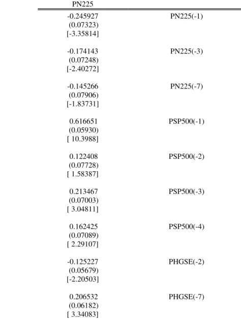
Table 13: Vector auto-regression of PN225 over lagged causal variables. Dependent Variable: PN225

Vector Auto-regression Estimates Sample(adjusted): 1/14/2009 9/16/2009

Included observations: 176 after adjusting endpoints Standard errors in ( ) & t-statistics in [ ]

PN225

PN225(-1) -0.245927

(0.07323) [-3.35814]

PN225(-3) -0.174143

(0.07248) [-2.40272]

PN225(-7) -0.145266

(0.07906) [-1.83731]

PSP500(-1) 0.616651

(0.05930) [ 10.3988]

PSP500(-2) 0.122408

(0.07728) [ 1.58387]

PSP500(-3) 0.213467

(0.07003) [ 3.04811]

PSP500(-4) 0.162425

(0.07089) [ 2.29107]

PHGSE(-2) -0.125227

(0.05679) [-2.20503]

PHGSE(-7) 0.206532

(10)

PFTSE100(-6) -0.130989

(0.06489) [-2.01855]

R-squared 0.466408

Adj. R-squared 0.437479

Sum sq. resids 0.033292

S.E. equation 0.014162

Akaike AIC -5.621402

Schwarz SC -5.441261

Mean dependent 0.001101