REM WORKING PAPER SERIES
Demographic Changes in a Small Open Economy with
Endogenous Time Allocation and Age-Dependent Mortality
João Pereira
REM Working Paper 063-2019
January 2019
REM – Research in Economics and Mathematics
Rua Miguel Lúpi 20,
1249-078 Lisboa,
Portugal
ISSN 2184-108X
Any opinions expressed are those of the authors and not those of REM. Short, up to two paragraphs can be cited provided that full credit is given to the authors.
Demographic Changes in a Small Open Economy with
Endogenous Time Allocation and Age-Dependent Mortality
Jo˜ao Pereira∗ 11th January 2019
Abstract
We calibrate an endogenous overlapping generations model of a small open economy to study the effects of population aging and population decline. In an invariant scenario public and foreign debt explode and GDP growth decreases markedly. Among the tested policies to control public finances, the best for the individuals is an increase in the retirement age, which needs to increase 6 years, a similar magnitude as the increase in life expectancy at birth. However, this increase has to happen before the increase in life expectancy materi-alizes itself. Aging has a stronger negative impact on public debt than population decline. We find a positive, but quantitatively modest, behavioral effect in reaction to a higher life expectancy with an impact on the GDP growth rate of only 2 basis points.
Keywords: Aging; Open Economy; Time Allocation; PAYG pensions; Debt. JEL Classification: J11; J22; H55; H63.
1
Introduction
People are living longer than ever and consequently, the World’s population is aging. Accord-ing to the United Nations (2015), the world’s median age will increase from 29.6 in 2015 to 36.1 in 2050 and 41.1 in 2100. Analyzing the aging process of advanced economies is partic-ularly relevant because they have usually a mature social security system that is sensitive to demographic changes. It is also important to quantify behavioral effects, i.e. the consumer’s reaction to a higher life expectancy, as that may mitigate the expected negative effects in the economy from an aging population.
With the purpose of performing this analysis, we developed in Guerra et al. (2018a,b) an overlapping general equilibrium endogenous growth model in order to study the transition dynamics of a small open economy affected by demographic changes. The consumer block, developed in Guerra et al. (2018b), shows consumers performing lifetime utility maximiza-tion, facing an age-dependent mortality law and allocating time freely at the intensive margin between leisure, learning, and work. The model includes a PAYG type pension system. The production sector developed in Guerra et al. (2018a) consists of a horizontal innovation endo-genous growth model. The model has two sources of growth: research and human capital, the latter because of a human capital externality introduced.
In this article, we perform the numerical simulation of that model. We calibrate the model with data from Portugal. Portugal is a good choice because it is a small open economy that is projected to have a strong population aging process. The model is run for a period spanning 50 years. The demographic data we use for this period is characterized by an increase in life expectancy at birth of approximately six years, a decrease in total population of 21.7% and an increase in the total dependency ratio of nearly thirty percentage points.
We have several goals. Firstly, to quantify the magnitude of this demographic change in the economy, mostly in terms of public and foreign debt, GDP growth but also at the con-sumer level, like the accumulation of human capital and labor supply. Another goal is to assess if in general equilibrium there exists a positive behavioral effect of the agents related to the increase in life expectancy and if so, how strong it is. Also, since we expect problems with debt sustainability, we want to test and compare several policies that can be used to keep public finances controlled. Finally, since our demographic scenario is characterized by both aging and a decreasing population, we would like to have an idea of the relative impact of each process. We should expect a big impact on the economy of this demographic change. This expect-ation is supported by evidence that shows a significant influence of demographic variables in the economy, but also because as we show in Guerra et al. (2018a), GDP per capita is affected negatively by a deterioration of the dependency ratio. This is in line with findings of, for example, S´anchez-Romero (2013), that in a study with endogenous labor supply and pensions applied to Taiwan, concludes that the demographic transition explains 22% of GDP per capita growth for the period 1965-2005. On the other hand, a recent study by Acemoglu and Re-strepo (2017) finds no evidence of a negative impact of aging on GDP per capita and suggests that technology adoption adjusts in a way that compensates for the potential negative effect of aging. Our model reveals an impact on GDP per capita, in particular in the period where the total dependency ratio adjusts the most.
The issue of whether there is a positive behavioral effect associated with aging has received a lot of attention in the literature. Hazan (2009) investigates if there is a Ben-Porath mechan-ism that connects life expectancy to an increase in human capital. He does this by noting that a necessary condition for this mechanism to exist is that lifetime labor supply should increase. Hazan computes a measure of this labor supply for the American population and notes that it decreased in time, which violates that necessary condition because life expectancy was rising. While Hazan used a fully rectangular survival law, Cervellati and Sunde (2013) generalize that analysis for an age-dependent survival law because a fully rectangular survival law does not capture changes in the survival law during working ages. Instead of Hazan’s necessary condition, they posit that the necessary condition for the Ben-Porath mechanism to exist is that increases in longevity raise the benefits of schooling relative to the opportunity cost of delaying the entry in the labor market. Data shows substitution effects from labor supply to schooling at younger ages, which is consistent with their necessary condition. They perform a numerical analysis that shows that is possible for an increase in longevity to simultaneously increase schooling and reduce lifetime labor supply.
Two recent panel data studies weigh in on a positive human capital effect on the economy arising from aging. Cuaresma et al. (2014) find that the demographic dividend is mostly an education dividend.1 Kotschy and Sunde (2018) project a strong negative consequence of aging for macroeconomic performance which could be compensated by human capital accumulation but estimate that human capital expansion might not be enough.
We also find a strong negative effect of aging on GDP growth and a positive behavioral effect, but the latter is not enough to compensate the former. This behavioral effect operates mainly through an increase in labor supply, with the increase in human capital being negligible. The article is organized as follows. The next section presents the calibration exercise. Sec-tion 3 explains the general numeric procedure. SecSec-tion 4 presents the results of the numerical simulation and Section 5 concludes.
2
Calibration
The model is run for a 50 year period, starting in 2020.2 We chose Portugal as the source of data to calibrate the model, because Portugal is a small open economy facing adverse demo-graphics. The calibration of the parameters was based on a mix of known values for Portugal and of the desired properties of the system in order to replicate empirical regularities. Much of this data is obtained from the AMECO database, which is the macroeconomic database main-tained by the European Commission’s Directorate General for Economic and Financial Affairs. As the model that we simulate is developed elsewhere (Guerra et al. (2018b) and Guerra et al. (2018a)), in Appendix B we present the relevant functional forms in order to allow for a
1
The demographic dividend is a concept that represents the positive effect on an economy of changes in the age structure of the population when the labor force grows at a higher rate than the population.
2
We do not perform a robustness analysis, running the model for different parameters as that is not our main goal. After we chose our base parameters we ran the model with them.
better understanding of the calibration exercise.
2.1 Consumers and Government
The parameters values from the consumer block are the ones used in the base scenario of the numerical simulation performed in Guerra et al. (2018b). All parameters used in our calibration are shown in Table 1. Regarding the government sector, we defined government consumption, G, as a fixed proportion of GDP. We chose it to be 17%. This value is in line with the historical average but is lower than recent values. The AMECO database shows an average of approximately 20% in the new millennium. We opted for the lower value because there are many government sources of revenue that we did not include in the model. Accord-ing to the Portuguese General Government Account for 2016, the weight of indirect taxes on GDP, excluding Value Added Tax (VAT), is 4.4%. By using a lower value for G/GDP we try to partially compensate for this absence.
Another tax that we do not have is VAT. VAT receipts evolve at the same rate as consump-tion so we included an updating rule in our lump sum tax (z0) in order for this tax to increase
at the same rate as the increase in consumption. In this way, the evolution of the lump sum receipts will be a bit closer to the evolution of VAT receipts in a real economy although it will still differ because of the impact of the population decrease. Since we had to fix this tax rate before we compute the consumption for each age cohort, this rule updates z0 with a one
iteration lag: z0(t) = z0(t − 2)∗ (C(t − 2)/C(t − 4)).3
For the corporate tax, we used a value of 22.5% which corresponds for the Portuguese corporate tax of 21.5% plus an average 1% municipal tax.
For the initial ratio of government deficit and public debt over GDP we opted to align it with the recommended goal of the EU’s Stability and Growth Pact, which sets a reference value of 3% for the deficit and 60% for the debt. So, we fixed the initial debt at that value. Regarding the deficit, after we defined the other fiscal parameters, we experimented with the lump sum tax, and fixed it at 0.0485 which results in an initial deficit of 2.1%, which is within the desired threshold.
As at the start of the simulation there will be already people retired, we needed to define how much each retired cohort was receiving in pension benefits. After computing the pension for the new retiree at the start of the model, we assumed every cohort was receiving a pension that was 4% lower than the immediately younger cohort, so the pension of people aged 82 at the start of the model was lower 4% than the pension of people aged 80. This assumes an average growth of new pensions of 2% per year. We chose this number because it is similar to the average growth rate of the wage rate displayed by the model and this is how much pensions should rise with a time invariant labor offer and human capital.
Although we had a goal for the initial deficit, we could not have one for the composition of government expenses in pensions and education. This happens because the way we model educational expenses is different from a real economy as we link a subsidy to time dedicated to
3
studying. This ends up putting a big weight on educational expenses as a percentage of GDP and is compensated by a lower weight of pensions over GDP than we observe for Portugal.
2.2 Capital
To compute the depreciation rate, we use the capital and investment series of AMECO and construct the depreciation rate for the period 1960-2019.4 This gives an average depreciation rate of 5.6%. We use the value of α = 0.35 which is the value that was used in constructing the series of AMECO, according to Havik et al. (2014).
In Guerra et al. (2018b) we explain why we set the low interest rate, r at 3%. The high interest rate rkand the parameter γ that defines the degree of substitutability between durable
goods were determined simultaneously. For this, we resorted to the total capital/output ratio (see Guerra et al. (2018a)) which is given by:
K + PAA
Y + PAA˙
= rk/p + (1 − tp)(1 − αγ) rk/α + (1 − tp)(1 − αγ)gA
Our idea was to define a capital-output ratio in the vicinity of 3 and to have the markup within Norrbin (1993) estimates. Several combinations were possible. We settled for γ = 1.95, that delivered an implicit rk of 7.1%. We decided to round it to 7% as this value also corresponds
to the average long-term return on equity reported by Mehra and Prescott (1985) for the USA and is used commonly in quantitative studies, two examples being Jones and Williams (2000) and Strulik (2007). The resulting markup is 1.465, on the upper limit of Norrbin’s findings.
2.3 Research Production Function
Calibration of the production function on research is slightly more complicated. We need to specify ξ, ζ, ϕA, T2020= A∗2020/A2020, A2020, and the exogenous growth rate of A∗.
We assume that, in our model, an economy at the frontier will have a research function with the same parameters as ours except for the catching up term, which vanishes. Through-out the calibration, we are going to use the United States of America (US) economy as the proxy for an economy at the technological frontier.
There is one aspect to take into consideration when calibrating the model with parameters deduced from the data. Our model is on a different scale, as time allocation is not defined in hours but as a percentage of total time. As such, aggregate human capital (H) is on a different scale than what we would obtain from the data. In the production function of the final goods sector, our scale parameter µ will make one of the necessary adjustments. Appendix E shows that, besides µ, only ζ needs to be scaled down. All the other parameters can be in the same magnitude as provided by the data.
AMECO’s data regarding TFP shows average annual growth rates of 1.9% and 1.1%, for PT and US, respectively. We assume that the economy at the frontier will share the parameter ϕAwith other economies, the only feature distinguishing them is the catching-up term. Then,
4
we did a similar exercise as in Jones and Williams (2000) to determine ϕA, but we needed to
interpret the TFP data in light of our model. Resorting to Havik et al. (2014) we see that TFP calculation is based on a production function that has as inputs capital and labor. The contribution of human capital is thrown into the TFP. Hence, we needed to extract from the TFP the contribution of human capital in order to have our TFP aligned with the one of AMECO. Since AMECO uses a production function of a final goods sector type, we compare it with our production function of that sector, implicitly assuming it represents GDP and therefore ignoring the contribution of the research sector, assuming, as seems reasonable, that it was small during the timeframe to which the data reports.
We will denote all growth rates by g. Using the expression for the production function of the final goods sector (6), the growth rate of the output of this sector is given by:
gY= (1 − α)gHY + (1/γ − α)gA+ αgK
If AMECO’s production function used human capital too we could simply say that gTFP =
(1/γ − α)gA, which is what Jones and Williams (2000) did. However, it is not the case. We
used an approximation of considering that our measure of human capital is labor force times hours worked times individual capital. Using the definition for H in (5), gH ≈ gLf+ gsw+ gh.
Because we are now aligning GDP by the production of the final goods sector, we assume gHY = gH. Then,
gY≈ (1 − α)(gLf+ gsw) +[(1 − α)gh+ (1/γ − α)gA]+ αgK
Now we can identify the expression inside squared brackets as similar to the TFP of the AMECO series obtaining:
gA≈ (gTFP− (1 − α)gh) (1/γ − α)−1 (1)
For gh, the growth rate of individual human capital, we used the Barro and Lee (2013) series
on average years of total schooling (population aged 15-64) for the period 1960-2010. The series is available with 5-year intervals and we used linear interpolation to fill in the gaps and also to extrapolate the series till 2019.
When obtaining the growth rate of A, we noticed that g∗A (US) still appears to be roughly constant after the human capital adjustment, so we proceeded like in Jones and Williams (2000), assuming the time derivative of g∗A is zero, setting ϕA= 1 − g∗HA/g∗A. If we call cA the
proportion of human capital employed in research, then HA = caH and we can approximate
gHA by:
gHA = gcA+ gH
≈ gcA + gLf+ gsw+ gh
Where we used the approximation to gHas before.5 For gsw we used the series regarding hours
of work from the OECD (2018a) (1960-2016). We also used OECD data (OECD (2018b)) re-garding employment in research. We use the rate of growth of employment in research as a
5
There is a slight abuse here. To match our expression of the TFP with the data, we assumed GDP was produced with the final goods sector production function, based on the assumption that the weight of the research sector was small during the period the data relates to. Nevertheless, now we take into consideration the change in the allocation of human capital to the research sector. We decided to do so, because our previous assumption was meant as an approximation and because there was, in fact, significant changes to the human capital employed in research since 1960.
proxy to our rate of growth of human capital employed in research (gcA).
6 Data is available
from 1981 to 2015, We extrapolated linearly the years from 1960 to 1980 based in the nearest growth rate and also the year 2016. Since the last data point for hours of work was 2016, we decided in both these series to not extrapolate it further till 2019. Regarding labor force we use data from AMECO again.
We obtain the following annual growth rates from the data for the US: g∗c
A = 0.01652,
g∗L
f = 0.0143, g ∗
sw = −0.00156, g∗h = 0.00567, g∗TFP = 0.01123. With this we obtain g∗H
A =
0.03493 and, with γ = 1.95 and α = 0.35, using (1) we obtain g∗A = 0.04634. As a result of this exercise we obtain ϕA ≈ 0.246, so we use ϕA = 0.25. This value is lower than the lower
bound in Jones and Williams, but we are factoring in human capital. The result goes in the direction of the study by del Barrio-Castro et al. (2002) in which they find that the elasticity of TFP to domestic R&D decreases markedly once human capital is taken into consideration. We need to specify an exogenous growth rate of ideas for the economy at the frontier. We do it by comparing its value with the one our economy will have. From the data, we obtain for PT, gh = 0.023545 and gTFP = 0.01904, resulting in gA = 0.023. This means that historically,
for the time frame we use, g∗A/gA= 2.018. The growth rate of ideas at the frontier has grown
approximately twice on average than the case of PT. This means that there has not been any convergence on the level of the stock of ideas, which seems at odds with our model, which implies a convergence with the frontier. However, if we use 5-year intervals data displays some convergence in the growth rate of ideas although not for the entire period. The difference between g∗A and gA has been decreasing.
When we calibrate the model, we have an initial growth of A of 5.87% so we set the exogenous growth g∗A = 11.74% which is twice the value of gA. This is much higher than
the historical rate but the model cannot replicate well levels of some variables, so instead of worrying with the level of g∗A we set it at a comparable ratio to gA.
We set T2020= 3.43 through a procedure, explained in Appendix D, that starts with a ratio
of GDP per capita by purchasing power between the US an Portugal, and works its way to a ratio of TFP and then to a ratio of A.
The remaining parameters were obtained jointly with the initial proportion of human capital dedicated to research. For this, we use the following three expressions for HY, gHY and
6
We cannot use employment in research to calibrate the level of our allocation to research. What our model allocates to research is human capital. Only because we take the simplifying assumption that average human capital is the same in research as in the sector producing the final goods, this allocation of human capital translates to an allocation of people. Nevertheless, to follow through with the calibration, we assume that the growth rate of employment in research provided by the data can be a good proxy to the growth rate of human capital employed in research.
gY¯, that are obtained in Guerra et al. (2018a): RMP A = rk(1 − α) (1 − tp)(1 − αγ)α(1 − cA)H gHY = gA− gRMP= cAH RMP A − ˙ RMP RMP = 0 gY¯= 1 − αγ γ(1 − α)gA+ gH(1 − α) + α(1 − cA)gHY 1 − αcA ≈ 0.015
Where RMP = ˙A/HA stands for real marginal productivity in research. Then:
RMP A =
[
ξAϕA−1+ ζ(T − 1)
]
And we used gHA = (gH− gHY(1 − cA))/cA to obtain the last expression.
These three equations are used to determine the unknowns from the research sector. We set the goal gHY = 0 as it is a neutral starting point and we want gY¯ (the GDP growth rate)
to be near 1.5% because it is AMECO’s estimate of the growth rate of potential output for Portugal for 2019.7
Nevertheless, we still have the problem of needing to estimate six unknowns (A2020, ξ, ζ,
cA, gH, H) with three equations. Hence, we further assume gH = 0, keeping the same neutral
stance we took for the goal for gHY, and we set ξ = 0.1 based on the literature, as we could
not find a satisfactory way to determine it.8
Now, we are still left with four unknowns for three equations. The determination of the parameters will depend on the initial level of H, which comes from the consumer maximization problem. This is a completely decentralized economy that required us to run the consumer problem in order to obtain H, but the result of his maximization problem will affect everything in the economy. We needed a value of H to determine the unknowns of the research function but at the same time, we needed the general equilibrium of the model to display similar ratios as a real economy and an acceptable initial government deficit. In fact, many of the values set for the parameters at the consumer level were chosen to take into consideration the desired properties at the aggregate while remaining within thresholds accepted by the microeconomic literature. We ran the simulation many times, making incremental changes in parameters be-cause every time we changed some parameter slightly all the consumer maximization changed. After several tries, we obtained a level of H = 1 213 490 that provides an initial equilibrium of the economy with the desired properties and satisfying gHY = 0 and with gY¯ = 1.47%. The
estimated values are A2020= 21 557 956, cA= 0.1 and ζ = 0.000000069.
7These growth rates we mention are instantaneous growth rates. When the simulation is run, the initial
growth rates will be slightly different, because we use a Runge-Kutta algorithm to integrate the set of equations ( ˙A, ˙D) at the aggregate level, and the right-hand side of the functions is influenced by the plans of the consumers.
8
We cannot compare our cAwith employment in research from data.9 It is naturally higher.
Only because we make the assumption that average individual human capital is the same re-gardless of the sector where it is being used, is that the allocation of human capital translates into an allocation of people. There are two reasons why it predicts more people employed in research than in reality. One is that on average, the human capital of a worker in research should be much higher than in the production of goods, but since the model has no hetero-geneity in human capital it will adjust by allocating more people to research. Also, the model assumes that human capital has a generic nature, can be applied anywhere and people with different human capital levels are substitutable. Since this is not true, this unaccounted het-erogeneity in the type of human capital acquired will also make cA higher than in the case
where human capital heterogeneity was accounted for.10 It is hard to see how someone with a PhD in Quantum Physics with, for example, 24 years of schooling, can be replaced by three dropouts from secondary school with 8 years of schooling each.
Although ζ looks very low, this happens because it is affected by the different scale in which our model is built. If we multiply our time allocation by the appropriate constant to make it annual, we will get the proper value of ζ that can be compared with models based on annual hours of work and study. In Appendix E we show that only ζ is affected by the scale factor in the research sector but also how to arrive at the proper constant c that we have to multiply to ζ to interpret it:
c = c
1−ϕη+ϕh 1−ϕη
s
Where csis the constant we multiply to the time allocation swand shin the consumer problem
to make it annual.
Since we use ϕh = 0.5 and ϕη = 0.01. This gives c = c1.505s . The highest value we can
consider for cs is 8 760 (24 hours, 365 days per year). With this, we have the true value of
ζ without the scale effect of approximately 0.06. This is the upper bound for ζ. In truth, it should be lower, because we cannot say people can freely choose between all three time activities during the full day, as there are physical limitations to that decision. Also, institu-tional aspects will make it lower, like the existence of a mandatory period of vacations or bank holidays.
The adequate results from the consumer were achieved with a wage rate of w = 4.5, ob-tained through experimentation. Since we need to have wy = wA and since wY depends on µ,
the latter was chosen as to equalize the two wage rates, resulting in µ = 0.179846776325242. This scale parameter, together with ζ are the only ones that are affected by the different scale of the model.
9
The OECD (2018b) reports for Portugal, in 2016, that employment in research activities is 0.88% of total employment.
10
Nevertheless, our result is a bit higher than what is usually found in other studies. Strulik (2007) gets a value of 6.34% for the decentralized equilibrium and 6.53% for the social planner, Funke and Strulik (2000) obtain 7.5%, Sequeira and Reis (2006) approximately 8% and Grossmann et al. (2015) in one of their scenarios obtain 10.4%.
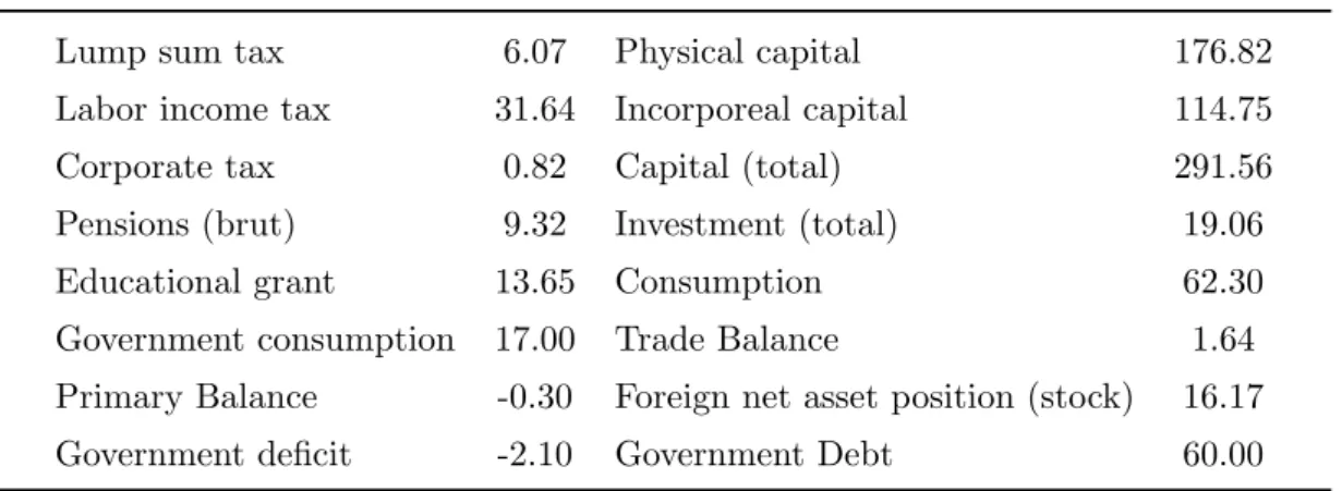
In the next table, we present the parameters used to run the model and in Table 2 some ratios at the start of the simulation.
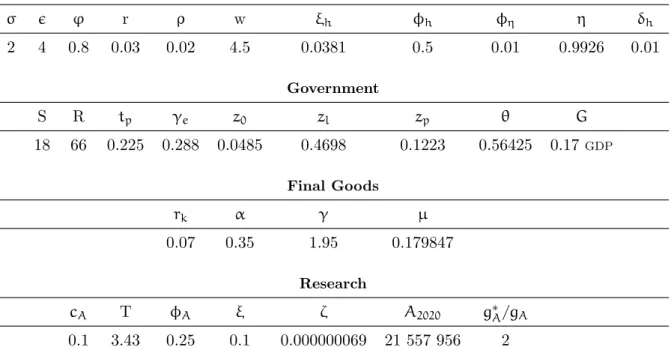
Table 1: Parameters and initial values of variables used in the numerical simulation
Consumer σ ϵ φ r ρ w ξh ϕh ϕη η δh 2 4 0.8 0.03 0.02 4.5 0.0381 0.5 0.01 0.9926 0.01 Government S R tp γe z0 zl zp θ G 18 66 0.225 0.288 0.0485 0.4698 0.1223 0.56425 0.17GDP Final Goods rk α γ µ 0.07 0.35 1.95 0.179847 Research cA T ϕA ξ ζ A2020 g∗A/gA 0.1 3.43 0.25 0.1 0.000000069 21 557 956 2
Table 2: Initial ratios % of GDP
Lump sum tax 6.07 Physical capital 176.82 Labor income tax 31.64 Incorporeal capital 114.75 Corporate tax 0.82 Capital (total) 291.56 Pensions (brut) 9.32 Investment (total) 19.06 Educational grant 13.65 Consumption 62.30 Government consumption 17.00 Trade Balance 1.64 Primary Balance -0.30 Foreign net asset position (stock) 16.17 Government deficit -2.10 Government Debt 60.00
3
Numerical procedure
The program is basically divided into two main blocks. One that computes the maximization problem of the consumers and another that computes the solution for each production sector, the government, and the remaining aggregate variables. We set the initial time in the year 2020 and run the model until 2070 with a grid of 2 years. This is the same grid for the age structure of the population. The population lives from age 0 to a maximum of 110 years. For this lifespan, they face a mortality function that they take into consideration when maximizing (Guerra et al. (2018b)). This means that, for each scenario we ran, we computed the lifetime optimization of 55 cohorts per year, for 25 times, representing 1375 consumer maximization problems per scenario. More details regarding the demography can be found in Appendix A.
Although we run the model with a grid of 2 years, the Runge-Kutta algorithm performs evaluations of the function at the midpoint of the step. In the case of the consumer block, we are also interested in the solution of the system of differential equations for this midpoint. In the Appendix of Guerra et al. (2018a) we show the adaptation made in the algorithm in order for it to compute the solution for the midpoint. This means that although we are running the model for 2-year intervals, we obtain the consumer plans with 1-year intervals. When we solve the consumer problem, we store the values of the variables for the present node (actual decisions) and for the next 2 nodes (planned decisions). Our main data file from the consumer block is comprised of data containing 9 columns (v, t, h, π, a, c, sl, sh, sw) for these 3 periods.
For every year, we start by computing the population’s maximization problem, given the wage rate and the human capital externality. The human capital externality depends on the average human capital of the previous period so we needed to set up an initial distribution of human capital per age at the start of the model. What we did was to run the full plan for a person at age 0 until age 110 and decide to set the distribution of human capital of the population similar to what that plan encompassed.11 After the population’s maximization
problem is solved we compute the program for the aggregate economy.
11
On the aggregate economy, we have a system of 2 differential equations on A and D that we solve using the same Runge-Kutta of fourth order. These functions depend on some variables that are the generational integration of the consumer variables. Since this algorithm evaluates the function at the initial node, at the end of the step but also performs mid step evaluations, we use now the values stored from the consumer block, the planned variables for the next two nodes. We do not integrate ˙K as K results from A.X.
Finally, due to the myopic expectations hypothesis, at the end of each iteration, we adjust the assets of the population, transferring dividends, the excess return on capital and profit/loss from the secondary market on patents to their balance sheets.
4
Results
4.1 Quantifying the problem
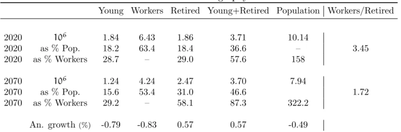
Table 3 presents information on the demographic transition that the economy will go through. This transition is characterized not only by aging but also by a decrease in population (21.7% in 50 years). By inspection of this table, it is easily understood why this will be a problem for a PAYG pension system. The number of workers per retiree decrease from 3.45 to 1.72, a cut in half. The total dependency ratio increases considerably from 57.6% to 87.3%. In terms of the dynamics of the model, we can guess the impact will have the fact that labor force is decreasing at an average rate of -0.83% per year, much higher than the average annual decrease of the population (-0.49%). The relative size of the labor force decreases 10 percentage points in the period.
Table 3: Demography
Young Workers Retired Young+Retired Population Workers/Retired
2020 106 1.84 6.43 1.86 3.71 10.14 3.45 2020 as % Pop. 18.2 63.4 18.4 36.6 – 2020 as % Workers 28.7 – 29.0 57.6 158 2070 106 1.24 4.24 2.47 3.70 7.94 1.72 2070 as % Pop. 15.6 53.4 31.0 46.6 2070 as % Workers 29.2 – 58.1 87.3 322.2 An. growth(%) -0.79 -0.83 0.57 0.57 -0.49
Source: Eurostat’s Population Projections Eurostat (2017). Data refers to the baseline scenario for Portugal.
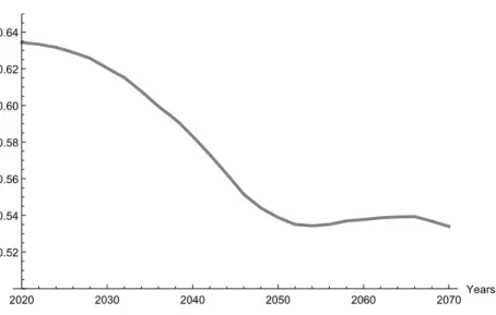
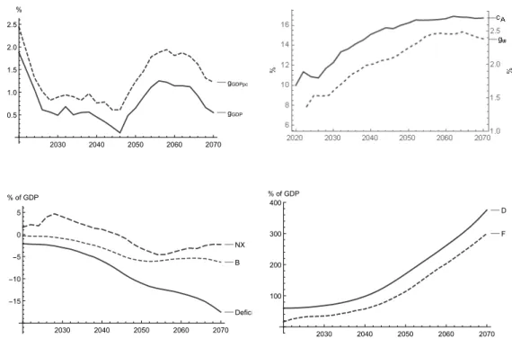
In Figure 1 we get to see that the movement of reduction of the relative size of labor force happens during the first 30 years until near the year 2050. After this period, the relative size of the population stabilizes at a new (lower) level. This seems to indicate that the biggest effect of the demographic transition will be felt in the first half of our simulation.
Figure 1: Labor force size relative to population 2020 2030 2040 2050 2060 2070 Years 0.52 0.54 0.56 0.58 0.60 0.62 0.64
happen if no policy would be taken. Then we compute several scenarios with different policies. We also ran a scenario without any demographic changes to use as a benchmark and few other artificial scenarios that are useful to illustrate some particular issues of the problem we are tackling.
Table 4 provides some descriptive statistics of the impact on the economy for the case of the invariant scenario. We started with a public debt position of 60% of GDP and it explodes to 375.4%. Similarly, we started with a fairly balanced foreign position, but foreign debt explodes too. This is a result of the increase in public debt as foreign trade is balanced on average. The human capital that appears in the table is the average individual human capital in phase 2 of the life-cycle, so it represents human capital supplied to the labor market. This measure is more relevant than the average human capital of the population. We see that it decreases annually and we see also that individual labor supply decreases.
Table 4: Impact on the economy
% GDP An. growth %
Average Deficit -8.55 GDP 0.75 Average NX -0.41 Pensions 0.62 D2070 375.4 human cap. -0.12
F2070 300.2 sw -0.29
GDP growth decreases, but what we are interested is in GDP per capita which, with a shrinking population is higher. GDP per capita growths at an average of 1.25%, which is still lower than the historical average since the 1960’s for Portugal, but this comparison may be displaced as the Portuguese economy had a strong convergence in the 1960’s. This growth is in line with the average since the 1990’s and even higher than in more recent years.
As a complement to Table 4, Figure 2 provides information about the evolution in time of some variables for the invariant scenario. We can notice that the big decrease in GDP happens in the period where occurs the big decrease in the relative size of the labor force (See figure 1). This happens because it is the period where gH is affected negatively the most. Once the
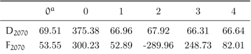
labor force stabilizes at a new proportion relative to the population, GDP growth recovers. We can also note the similarity of the trajectory (and of the concavity) of the growth rate of w (labor productivity) with the evolution of human capital allocated to research. Trade Balance deteriorates but recovers a bit towards the end. Its evolution is no cause of concern. Regarding public finances, the economy starts with a primary balance of almost zero, but it deteriorates continuously reaching levels of 5% to 6% more or less at half of the period simulated and never recovering from that. As a consequence, the deficit continuously deteriorates, reaching a value of -17.52% at the end of the simulation. The deterioration of the deficit causes public debt to explode and this leads to an explosion of foreign debt.
Figure 2: Invariant scenario with demographic transition
gGDP gGDPpc 2030 2040 2050 2060 2070 0.5 1.0 1.5 2.0 2.5 % NX B Deficit 2030 2040 2050 2060 2070 -15 -10 -5 0 5 % of GDP D F 2030 2040 2050 2060 2070 100 200 300 400 % of GDP
The invariant scenario reveals the full extent of the problems arising from the demographic transition for our small open economy. It is, clearly, a scenario that is not feasible as in the real world international capital markets would demand higher interest rates as soon as signs of loss of control of public finances appeared. This would exacerbate the problem and, at some point, the international capital market will completely dry up, with everybody refusing to lend to this government. A rescue plan would need to be put in place, which would require the government to implement harsh policies to control the deficit. The scenario shows, then, the inevitability of action by the government, either voluntarily or imposed.
We also computed a scenario without demographic transition, in which the total popula-tion, the age structure, and the mortality rate remained constant throughout the simulated period. In this scenario, public debt increases from 60% to 69.5% by 2070 and foreign debt increases from 16.2% to 53.6%. It is a very small increase in public debt for a 50 year period. It means that, without demographic transition, the economy is basically balanced in what regards public finances and that the debt explosion can be attributed to the demographic transition.
We use this constant demography scenario as a benchmark. In the several policy experi-ments we make, we try to get public debt by the year 2070 at a similar level to the one obtained with constant demography. As we have to run the entire population’s consumer problem every two years, we will be satisfied with final debt levels in some reasonable neighborhood of this benchmark. Beyond some point, the time spent running the simulations is not worth it, as a finer tuning of the final debt ratio does not bring extra insights.
4.2 Policy experiments
We test four ways in which the government can act to control the deficit. An increase in labor income tax, a decrease in the replacement rate, a decrease in the educational subsidy and an increase of the retirement age. For the remaining of this article, it will be useful to name all scenarios with numbers. Naming the scenarios is useful because it eases the exposition and brings clarity. Later, when we mention, for example, scenario 12, it will be easily understood as a combination of scenario 1 and 2, or 234 as a combination of 2, 3 and 4:
0. Invariant with demographic changes. 0a. Invariant without demographic changes.
1. Labor income taxes increase linearly 0.26 percentage points per year.
2. Replacement rate decreases linearly until it reaches zero in 2054. It represents a decrease of approximately 1.66 percentage points per year.
3. Educational subsidy decreases linearly approximately 0.37 percentage points per year. 4. Retirement age increases six years: to 67 in 2022, 68 in 2026, 69 in 2030, 70 in 2034, 71
in 2040, and 72 in 2046.
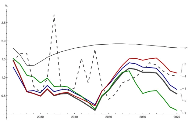
The level of the changes in policy in each scenario was obtained through experimentation as we cannot determine a priori the required changes in policy. All of them manage to keep public debt under control. The next table summarizes the results.
Scenario 3 and 4 deserve an introduction. Scenario 3 is a scenario that makes sense in our model because educational expenses are an important public expense but are not comparable to a real economy because educational expenses are linked to the wage rate and time dedicated to studying. In this expense, the wage rate is multiplied by the educational subsidy rate and by the time dedicated to studying. Since the wage rate increases every year and it increases at a higher rate than GDP, if there is not a sufficient decrease in the time allocated to schooling,
Table 5: Debt results by type of policy instrument % of GDP
0a 0 1 2 3 4
D2070 69.51 375.38 66.96 67.92 66.31 66.64
F2070 53.55 300.23 52.89 -289.96 248.73 82.01
the weight of educational expenses on GDP will grow. What this scenario does is to reduce γe at a rate not very different of the increase in w. It acts as a brake on the increase of
educational expenses.
In the case of scenario 4 we realized, not surprisingly, that increasing the retirement very early in the simulation is more effective in reducing the debt. Basically, the increase in the retirement age has to be preemptive as it needs to occur before the increase in the life expect-ancy. The demographic data from Eurostat project an increase in life expectancy at birth of 6.16 years during this period and an increase of 4.56 years in life expectancy at age 65. This scenario increases the same number of years as the increase of life expectancy at birth. This is not the only configuration possible for the years where we chose to increase the retirement age. The important thing to happen is that it really needs to have a strong emphasis at the start of the simulation although some variation on the years can reach a similar result.
Portugal reformed its pension system to include a sustainable factor that links the evolu-tion of the retirement age to changes in life expectancy at age 65. In our model, this would not be enough, because we needed to increase the retirement age by 6 years.
Scenario 2 represents not only a cut in pensions, but pensions also have to be reduced to zero by 2054. Relying only upon this instrument means that the PAYG pension system has to be terminated.
Although all policies tested are successful in controlling public debt, scenario 3 fails to control foreign debt. This happens because the educational subsidy also represents the source of income in the first phase of the life-cycle. When it is reduced it will affect the differential equation of assets right at the start, interfering with its accumulation, leading to a much lower level of individual assets throughout the life-cycle. At the aggregate level, the private savings of the population will be much lower and capital stock needs to be financed with international funds.
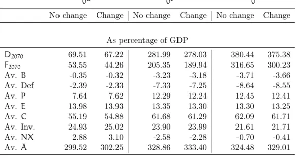
In Figure 3 we show how the scenarios compare in terms of GDP growth rate and we include the scenario without demographic changes that serves as the benchmark. All of them display a decrease in the growth rate until 2046. It is interesting to compare this result with figure 1 as it shows that the biggest impact in growth happens while the transition of the relative size of labor force unfolds.
Scenarios 1, 2 and 3 display very similar growth rate trajectories as scenario 0 although with different levels. Scenario 4 displays discrete jumps because of the discrete increases in
Figure 3: GDP growth rates 0 0a 1 2 3 4 2030 2040 2050 2060 2070 0.5 1.0 1.5 2.0 2.5 %
the retirement age. But it is clear that the growth rate of scenario 4 is, on average, the highest from all policy scenarios considered.
We could take GDP per capita growth as a criterion to rank these alternatives, which boils down to compare GDP growth as population growth is the same. GDP per capita is good as an indication of standards of living. However, there is a better criterion. In the end, what everyone wants is to be happy and it is the government’s duty (or should be) to ensure it can be achieved as much as possible in a sustainable way. Therefore, we measured the impact of each scenario on the population’s utility.
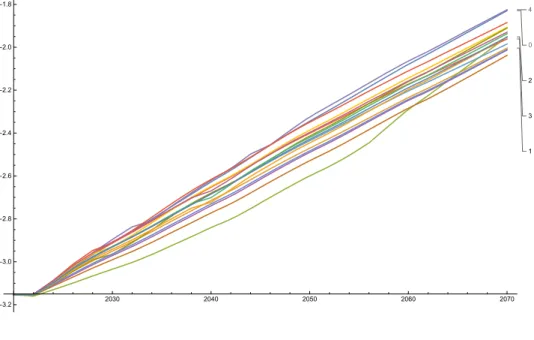
We computed the instantaneous utility for each cohort of the population and computed a weighted average for each year. In all scenarios utility growths in time with not relevant crossing points (See Appendix E.1), which allows us to compare the relative merit of each policy by comparing the average population’s utility during the period.
We now introduce policy mix by combining several instruments. We had four instruments and we conjugate them 2 by 2, 3 by 3 and one scenario with all instruments. There is an infinite range of possibilities to combine them but we just explored one linear combination. The additional scenarios computed are:
12. Half of the adjustment in 1 and half of the adjustment in 2. Labor income taxes increase 0.13 percentage points per year and the replacement rate decreases approximately 0.83 percentage points per year.
decreases approximately 0.19 percentage points per year.
14. Adjustment in 1 like in 12 and retirement age increases three years: to 67 in 2022, 68 in 2030 and 69 in 2034
23. Adjustment in 2 like in 12 and adjustment in 3 like in 13. 24. Adjustment in 2 like in 12 and adjustment in 4 like in 14. 34. Adjustment in 3 like in 13 and adjustment in 4 like in 14.
123. One-third of the adjustment in 1, one-third of the adjustment in 2 and one-third of the adjustment in 3. Labor income taxes increase approximately 0.09 percentage points per year, the replacement rate decreases approximately 0.55 percentage points per year and the educational subsidy decreases approximately 0.12 percentage points per year. 124. Adjustment in 1 and 2 like in 123 and retirement age is increased two years: to 67 in
2022 and to 68 in 2040
134. Adjustment in 1 and 3 like in 123 and in 4 like in 124. 234. Adjustment in 2 and 3 like in 123 and in 4 like in 124.
1234. One-fourth of the adjustment in 1, 2 and 3 and retirement age is postponed only one time, to 67 in the year 2022. Labor income taxes increase approximately 0.07 percentage points per year, the replacement rate decreases approximately 0.41 percentage points per year and the educational subsidy decreases approximately 0.09 percentage points per year.
The results of these policies are presented in Table 6.12 The scenario 0a, which is the scenario with a constant demography is useful to study some properties of the model. For example, all scenarios show negative average growth rates in human capital and labor supply and part of this could be attributed to changes in the age structure of the population, but even in scenario 0athis happens. A reduction on human capital and labor supply is also a response of consumer’s to a higher wage rate, an effect we observed in the partial equilibrium analysis of Guerra et al. (2018b) and which is now confirmed in general equilibrium. Regarding labor supply, our results are not far from the historical trend. Data from the OECD (2018a) show an annual growth of hours worked for Portugal of (−0.256%).
As equation (9) shows, GDP growth is the sum of the growth in the wage rate (productiv-ity) plus a term that is a function of the difference between the growth of total human capital and the growth of human capital applied to research and the size of the allocation of human capital to the research sector. In all scenarios GDP growth is lower than the growth in w because that second term in our simulations has always a negative contribution. Total human capital grows at a negative rate because individual human capital and labor supply grow at a negative rate. This is compounded on the scenarios with demographic changes as labor force grows also at a negative rate. Human capital applied to research, however, can grow at a positive or negative rate but this rate is always higher than the growth rate of total human
12In Table 6, averages are computed for the period 2020-2070 and h
2 refers to individual human capital in
capital because we observe in all scenarios an increase in the allocation of human capital to research.
In the theoretical case of a BGP, which requires no changes in the age structure of the population, but in which population can grow, there would be a constant allocation of human capital to research. In this case GDP growth (equation (10)) would still be lower than the growth of w, due to the substitution of study and labor for leisure by consumers, unless the growth rate of the population was sufficiently strong.
In the scenario without demographic changes, labor productivity which is determined by the productivity in research, grows at a rate of 2.28% per year. If we subtract -0.44%, which is the growth in total human capital (-0.13% from the individual human capital and -0.31% from labor supply) we obtain 1.84%. The growth of potential output is slightly lower (1.76%) due to the effected of the increase in the proportion of human capital allocated to research.
In the invariant scenario (0), productivity grows at 2.09% and GDP at 0.75%, meaning that this adverse demography costs the economy 21 and 101 percentage points per year in productivity and GDP growth, respectively. In scenarios in which we test policies to keep the debt under control, GDP tends to grow at a higher rate because consumers react to these measures, that impact negatively consumption, by working more hours. In some scenarios there is also an increase in the time allocated to learning, resulting in increases in human capital when comparing with the invariant scenario.
Although our model presents a very stylized version of a small open economy calibrated with data from Portugal, it is somewhat reassuring that the 2018 Ageing Report from the European Commission (DG-ECFIN (2018)) estimates an annual GDP growth rate of 0.9% for an invariant scenario that includes only the automatic update of the sustainability factor, which sits between our growth rate for the invariant scenario of 0.75% and the growth rate of 1.1% for the scenario with the increase in the retirement age.
T able 6: Selected indicators for all scenarios 0 a 0 1 2 3 4 12 13 14 23 24 34 123 124 134 234 1234 As % of GDP D2070 69.51 375.38 66.96 67.92 66.31 66.64 60.52 64.76 70.87 62.22 77.07 81.29 62.52 62.88 63.62 69.07 80.07 F2070 53.55 300.23 52.89 -289.96 248.73 82.01 -124.86 151.52 86.66 -19.98 -60.37 194.40 3.41 -31.79 138.95 40.42 56.21 Av. B -0.35 -3.66 0.59 0.97 1.06 0.08 0.88 0.87 -0.05 1.09 0.16 0.15 0.95 0.43 0.46 0.55 0.21 Av. Def. -2.39 -8.55 -1.44 -1.31 -1.04 -1.56 -1.24 -1.19 -1.85 -1.09 -1.84 -1.78 -1.17 -1.52 -1.43 -1.49 -1.90 Av. P 7.64 12.41 12.20 6.73 12.17 9.05 9.35 12.17 11.15 9.35 8.47 11.14 10.29 9.60 11.35 9.60 10.67 Av. E 13.98 13.25 13.32 13.00 8.52 12.16 13.11 10.89 12.82 10.72 12.65 10.50 11.57 12.79 11.36 11.25 11.86 Av. C 55.19 61.71 57.46 54.66 59.06 56.63 55.47 58.22 57.24 56.27 56.08 58.17 56.65 55.96 57.51 56.55 57.14 Av. In v. 24.93 21.71 22.11 21.97 22.28 21.58 22.30 22.22 20.19 22.40 20.23 20.27 22.31 20.87 20.87 20.92 20.30 Av. NX 2.88 -0.41 3.43 6.36 1.66 4.79 5.23 2.56 5.57 4.33 6.69 4.57 4.04 6.17 4.63 5.53 5.57 Av. ¯ A 299.52 329.01 301.74 423.32 246.58 284.80 361.62 273.82 289.05 334.03 344.65 261.99 323.13 328.40 272.57 310.48 309.02 Ann ual gro wth rates (%) GDP 1.76 0.75 0.85 0.74 0.92 1.11 0.85 0.89 0.96 0.90 0.95 0.99 0.88 0.95 0.98 0.98 0.91 w 2.28 2.09 2.11 2.09 2.12 2.16 2.11 2.11 2.14 2.11 2.14 2.15 2.11 2.14 2.14 2.14 2.13 P/GDP -0.81 0.62 0.54 -4.25 0.46 -0.19 -0.96 0.49 0.35 -1.01 -1.22 0.31 -0.36 -0.56 0.31 -0.59 -0.11 E/GDP 0.16 0.19 0.19 0.23 -2.12 -0.09 0.17 -0.69 0.08 -0.71 0.06 -0.80 -0.37 0.08 -0.46 -0.47 -0.26 C 1.39 0.76 0.52 0.57 0.61 0.83 0.47 0.57 0.67 0.52 0.66 0.72 0.52 0.60 0.65 0.64 0.60 Consumer v ariables Av. h 0.458 0.458 0.460 0.458 0.458 0.463 0.459 0.459 0.462 0.458 0.461 0.461 0.459 0.461 0.461 0.460 0.460 gh (%) -0.12 -0.13 -0.11 -0.14 -0.12 -0.08 -0.12 -0.11 -0.09 -0.13 -0.10 -0.09 -0.12 -0.10 -0.10 -0.11 -0.11 Av. h2 0.518 0.518 0.521 0.517 0.519 0.522 0.519 0.520 0.522 0.519 0.521 0.522 0.519 0.521 0.521 0.520 0.520 gh 2 (%) -0.13 -0.12 -0.10 -0.14 -0.10 -0.09 -0.12 -0.10 -0.09 -0.12 -0.11 -0.09 -0.11 -0.11 -0.09 -0.11 -0.11 Av. s w 0.337 0.340 0.343 0.351 0.345 0.333 0.349 0.344 0.337 0.349 0.342 0.338 0.347 0.343 0.340 0.343 0.343 gs w (%) -0.31 -0.29 -0.24 -0.29 -0.17 -0.33 -0.21 -0.20 -0.28 -0.18 -0.27 -0.25 -0.19 -0.25 -0.24 -0.23 -0.22 Av. util. -2.532 -2.496 -2.593 -2.668 -2.544 -2.486 -2.638 -2.569 -2.531 -2.611 -2.553 -2.504 -2.605 -2.573 -2.537 -2.555 -2.561 gutility (%) 1.07 1.07 0.90 0.94 0.94 1.08 0.86 0.91 0.99 0.89 0.99 1.02 0.89 0.95 0.97 0.96 0.95
We can observe that, with some varying degree of success, all tested policy mixes manage to control public debt. There is a slight loss of traction in scenarios 24, 34 and 1234. Regarding the policy mixes we tested, their results, presented in Table 6, are also combinations of the base scenarios. That is why, from the perspective of controlling the public debt, there are no reinforcing effects from combining different instruments. There are, however, complementarity effects in what regards foreign debt. Scenario 2 produced a strong positive foreign position while scenario 3 failed to control foreign debt. By combining them, scenario 23 produces a satisfactory result both on public debt and on the foreign position. When scenario 3 is com-bined with other scenarios that do not involve scenario 2, foreign debt is not controlled in a satisfactory way.
The worst policy for the consumers is a cut in pensions (scenario 2), as this is the case where the average utility of the population is lower. Cutting pensions is also the scenario where productivity and GDP grow at a lower rate even taking into consideration that it is the scenario with the higher average labor supply.
The best policy for the population is an increase in the retirement age (scenario 4). Al-though this scenario does not perform so well in terms of foreign debt it performs better in many other domains. Besides being the scenario where average utility is higher, it is also the scenario where average utility grows at a faster rate. It is the policy that results in a higher growth rate of productivity and GDP because it is the one with the strongest effect on human capital accumulation.13
From the analysis we performed, just increasing the retirement age is the best policy, unless there are no extra concerns regarding foreign debt. If we would like to see a lower level of foreign debt in 2070, we have to consider one of the scenarios that end with a level of foreign debt not much higher than the benchmark scenario (23, 24, 123, 124, 234, 1234). Using the criteria of average utility, the best is 24, which is a combination of a cut in pensions and an increase in the retirement age.
4.3 Population decrease versus change in the age structure
In this section, we try an exercise that can help to shed some light on the relative magnitude of the difficulties posed by the decrease of the total population and by the change in the age structure. We compute a scenario in which aging occurs (the age structure changes) but we keep total population constant. We take the population dataset and compute the weights of the cohorts in total population from 2020 to 2070. After we assume that total population stays constant at the 2020 level and compute the new population per age with those weights.
14 This scenario is the one labeled (0c - Change) presented in Table 7 in the next subsection.
13
Average h2may be influenced by the way average is calculated, as the active life period keeps expanding, but
we can also see that it is the scenario with the highest average human capital regarding the entire population.
14There is a technical issue here as the exercise was done in order for the sum of all age population, obtained
from the data, to be the same every year, but since these are densities that we integrate, there are slight variations in the total population. However, this should have a very little impact on results and for the type of analysis we perform here, are irrelevant.
In the invariant scenario, the government debt deteriorates from 60% in 2020 to 375.38% in 2070, an increase of 315.38 percentage points. With the current scenario, government debt rises to 278.03% in 2070, a 218.03 percentage points increase. Hence, the change in age struc-ture has more impact on government debt than the decrease in the size of the population. Once we control for the population size, 69% of the initial deterioration still unfolds. The decrease in the size of the population has a slightly bigger impact on foreign debt but similar conclusions can be drawn regarding the relative importance of changes in the age structure. Foreign debt now rises 173.78 percentage points, approximately 61% of the initial deterioration. This analysis shows also that relying only on replacement migration to solve the demo-graphic problem has a limited effect. Nevertheless, if the median age of migrants is younger than the age of the resident population, migration will also cause some impact on the age struc-ture. This is usually what happens as migration is frequently motivated by families searching for a better country to live and work.15 Summing up, the contribution of migration will be higher, the younger migrants are.
4.4 The behavioral effect
An increase in the life expectancy will increase the dependency ratios, putting pressure on the pension system. There will be a lower proportion of the population producing goods and services supplied to the market. This is the accounting effect of aging. Nevertheless, economic literature suggests that there should be a positive behavioral effect in the sense that people should react to a higher life expectancy by working more and investing more in human cap-ital, becoming in this way, more productive. This positive effect can mitigate the negative accounting effect. In Guerra et al. (2018b), in a partial equilibrium analysis, we showed the existence of this positive effect. However, we need to study what happens in a general equi-librium analysis, as consumer decisions impact the firm’s decisions, not only in what regards the production of goods but also on research. We also need to quantify it, because we would like to have a reasonable estimate of its magnitude.
The scenarios we computed already have an eventual behavioral effect accounted for be-cause we let the mortality rate change. In this way, the invariant scenario (0) in which public debt explodes, already demonstrates that if this effect exists, it is not enough to counteract the negative effects of aging.
The exercise we performed was to recompute some scenarios but now using the same sur-vival function for the whole period.16 By comparing the scenario in which the survival function changes with the scenario in which it doesn’t, we can attribute the differences to the reaction of the consumer’s to a higher life expectancy. In Table 7 we present the cases for the scenario
15
The scenario tested in this section could be considered a case in which there was a sufficient extra influx of migration to avoid a decrease in population with the implicit assumption that the age distribution of migrants is the same as the resident population. However, the comparison is not straightforward as migrants with age over 66 would not be a burden for the pension system as they would be receiving a pension from their home country.
without demographic transition (0a), the scenario that allows changes in the age structure but
without a decrease in the population size that was analyzed in the previous subsection (0c) and the policy invariant scenario (0).
Table 7: Comparing scenarios with and without changes in the mortality law
0a 0c 0
No change Change No change Change No change Change
As percentage of GDP D2070 69.51 67.22 281.99 278.03 380.44 375.38 F2070 53.55 44.26 205.35 189.94 316.65 300.23 Av. B -0.35 -0.32 -3.23 -3.18 -3.71 -3.66 Av. Def -2.39 -2.33 -7.33 -7.25 -8.64 -8.55 Av. P 7.64 7.62 12.29 12.24 12.45 12.41 Av. E 13.98 13.93 13.35 13.30 13.30 13.25 Av. C 55.19 54.88 61.68 61.29 62.09 61.71 Av. Inv. 24.93 25.02 23.90 23.99 21.61 21.71 Av. NX 2.88 3.10 -2.58 -2.28 -0.70 -0.41 Av. ¯A 299.52 302.25 328.86 333.40 324.48 329.01
Annual growth rates(%)
GDP 1.76 1.78 1.31 1.33 0.73 0.75 w 2.28 2.28 2.19 2.19 2.08 2.09 P/GDP -0.81 -0.81 0.57 0.56 0.63 0.62 E/GDP 0.16 0.14 0.22 0.20 0.20 0.19 C 1.39 1.39 1.31 1.31 0.76 0.76 Consumer variables Av. h 0.458 0.458 0.458 0.458 0.458 0.458 gh (%) -0.12 -0.11 -0.13 -0.13 -0.13 -0.13 Av. h2 0.518 0.518 0.518 0.518 0.518 0.518 gh2 (%) -0.13 -0.13 -0.13 -0.13 -0.13 -0.12 Av. sw 0.337 0.338 0.338 0.340 0.339 0.340 gsw (%) -0.312 -0.302 -0.312 -0.301 -0.304 -0.294 Av. util. -2.5322 -2.5322 -2.4768 -2.4826 -2.4899 -2.4957 gutility (%) 1.07 1.07 1.11 1.11 1.08 1.07
We may observe that this positive effect exists and operates mainly via an increase in labor supply. There is also a very slight increase in the average human capital but is not visible at 3 decimal points. Labor supply still decreases as a result of the increase in the wage rate but decreases at a slower pace. As a result, the growth rate of the stock of ideas (not shown) is 2 basis points higher, the investment rate is 9 basis points higher (10 basis points in the
invariant scenario) and GDP grows 2 basis points higher.
At the end of the 50 year period that we ran the model, the government’s debt and foreign debt are lower, but not by much, with the impact being even more modest in the government’s debt than in the foreign debt. For the invariant scenario (0), the behavioral effect has a pos-itive impact of public debt in 2070 of approximately 5 percentage points. We conclude that this positive effect exists but is quantitatively small.
4.5 The model and the real world
In this section, we discuss how the results of this article could compare with a real economy. Some of the hypothesis used for simplification may cause an overestimation of the problems arising from an adverse demographic transition, while others may cause an underestimation. This is a highly simplified version of an economy so we will just focus on a few aspects of the model.
Our output is potential output obtained with zero unemployment. In the real world, even if the economy is at full employment, there will always be unemployment. The way potential output is estimated by economists includes some percentage of the unemployed population. In the real world, the economy is subject to business cycles and crisis. The deeper the crisis, the heavier the extra weight put on public finances. For example, in the recent great recession originated by the US subprime mortgage crisis, Portugal needed an international bailout and the unemployment rate rose from 9.1% in 2007 to a peak of 16.4% in 2013. These high levels of unemployment are not accounted for in our model, causing the model to underestimate problems of debt financing.
Another source of underestimation is that we rely on a demographic scenario that includes an estimate of migration. If migration is lower than projected, the public debt problem will be more acute. Also, we consider no heterogeneity in human capital but is reasonable to assume that a relevant proportion of immigrants have lower human capital than the resident population, as many come from less developed countries in search for higher salaries. On the other hand, higher migration rates than projected, improve the demographic scenario. We saw above the if population decline was prevented, the debt explosion would reduce in nearly one third. Furthermore, migrants tend to be younger, on average, than the resident population. An important assumption is the initial level of the government debt to GDP ratio. We started with 60%. If we started with double this value, which is, for example, the case in Portugal, debt dynamics would make the goal of keeping debt sustainable harder to achieve.
On the positive side, a feature of the model that may be overestimating the problem, is the fact that not everybody can adjust labor supply downwards because most workers have labor contracts stipulating some minimum amount of hours of work. Our hypothesis of free allocation of time was made to enhance the behavioral effect, but it applies more realistically to the self-employed population. This means that, as a reaction to an increase in the wage
rate, we should expect labor supply at the intensive margin to decrease at a slower rate.17 GDP should grow at a faster rate.
Also, the behavioral effect is probably stronger than computed, because the survival laws we used, result in a smaller increase in life expectancy than the one implicit in the age struc-ture of the data. Plus, we only changed the survival law every 10 years, with the first change occurring only in 2030.
More important, are the simplifications we took with the government sector. We assumed in the model that the entire population has the same rule for determining the pension benefit. In reality, there are subsets of the population with different rules, many of them more favorable than the general rule. If these subsets are big, they will cause additional problems in financing social security.18 We did not include several taxes, like the VAT or excise duties in mineral oils, tobacco and alcohol. With fixed tax rates, the revenues from the VAT, and in some degree, excise duties, should grow at a similar rate as consumption. We implemented a rule that makes the lump sum tax rate to grow at the same rate as private consumption, but lump sum revenues are still affected by the growth rate of the population, which is negative. Therefore, our lump sum revenues are growing at an annual rate of that is the growth rate of consumption (the growth rate of VAT) minus 0.49%, which is underestimating annual government revenues.
5
Conclusion
In this paper we ran numerically a general equilibrium model developed in Guerra et al. (2018a,b). We tested the impact over a period of 50 years of a demographic transition. Over this period, total population decreases 21.7% and the proportion of the labor force decreases 10 percentage points.
With constant demography, the economy would have sustainable debt as both public and foreign debt increase moderately. However, with demographic changes and in case the gov-ernment does nothing, both public and foreign debt would explode. GDP growth is hit the hardest during the relative decrease in the proportion of the labor force. Once this proportion stabilizes in a new lower level, GDP growth recovers somewhat.
The government’s policies that we test are an increase in social security contributions, a cut in pensions, an increase in the retirement age and a cut in educational expenses. All these alternatives manage to keep government debt sustainable and with the exception of the cut in educational expenses. They also keep foreign debt sustainable. We also test some linear combinations of these policies and they also manage to control the government’s debt. There is some complementarity in cutting pensions and cutting educational expenses in what regards foreign debt, as cutting pensions has a strong effect in moving the economy towards a net creditor position, and in this way compensates for the poor result that cutting educational
17
In the invariant scenario, it decreased an average of -0.31% per year.
expenses has in this variable.
We use the population’s average utility as a ranking criterion among these options. The most penalizing policy for the consumer is the cut in pensions and the least penalizing is the increase in the retirement age. Relying solely upon the increase in the retirement age is also better in several other dimensions. It is the policy in which consumers decide to accu-mulate more human capital, delivering the highest productivity and GDP growth amongst the alternatives we tested. Nevertheless, it was necessary to increase the retirement age 6 years, during the first half of the 50 year period of the simulation. The data we use has an implicit increase in life expectancy at birth of 6 years during that period. To be effective, the increase in the retirement age can be of a similar magnitude as the increase in life expectancy at birth but has to be implemented preemptively. If we didn’t concentrate the increase in the first half of the simulated period we would not have been able to control the government’s debt. We also analyze the relative impact of the decrease in the population size and the change in the age structure on debt explosion and conclude that roughly 2/3 can be attributed to the change in the age structure and 1/3 to a decline in the population.
Finally, we assess the quantitative importance of the behavioral effect, the consumer reac-tion to a higher life expectancy. We observe that this effect exists at the general equilibrium level and operates mainly through an increase in labor supply with negligible effects in hu-man capital accumulation. It is, however, quantitatively small. In the scenarios we tested, it increased the investment rate by 9-10 basis points, GDP growth by 2 basis points and in the invariant scenario, its impact on the government debt at the end of the simulation was only of 5 percentage points. The behavioral effect may be biased downwards because of some decisions made regarding the numerical program, but it should sit still too far to significantly counteract the deterioration of the dependency ratios.
Appendix
A
Demography
The population age distribution we use is taken from Eurostat’s baseline population projec-tions for Portugal by (Eurostat (2017)). We run the full model of the economy for the years 2020-2070 based on them. The projections include population by age composition till age 99 and a class defined 100+. We interpolated the values till age 110. Population by age was divided by 2 years intervals. Regarding the mortality function we computed initially two mor-tality functions. One for the year 2015 based on data from the Human Mormor-tality Database (2017) and another for the year 2080 based in Eurostat’s projections.19 Then we linearly inter-polated between these two to obtain mortality functions for 2020, 2030, 2040, 2050 and 2060. To simplify the computation process, we decided to not change the mortality function every year. Instead, we used the one from 2020 to compute the consumer maximization programs for the years 2020 to 2028, the one from 2030 was applied from 2030 to 2038, the mortality rate
for 2040 was applied from 2040 to 2048, the one for 2050 was applied from 2050 to 2058 and the mortality computed for 2060 was applied from 2060 to 2070. For the partial equilibrium analysis in Guerra et al. (2018b) we used the mortality functions estimated for 2020 and, for the examples with a higher life expectancy, the one estimated for 2080.
When we computed the mortality function with the data for 2080, we realized that the probability of surviving age 110 was close to zero but not so close as we would like it to be. Since the mortality function enters as integrand in several integrals and since we use a cutoff at age 110 on integrals that are analytically defined to infinity, we need this probability to survive age 110 as close to zero as possible in order to avoid significant numerical errors. So we changed slightly the function we computed in Mathematica in order to achieve this. This change has the side effect that the aging those mortality functions display is milder than the aging that Eurostat has implied and, therefore, there is a mismatch between the aging the structure of the population reveals and the aging that consumers take into consideration when optimizing.20 Nevertheless, everything considered, we decided to proceed with the change as we preferred to minimize numerical errors on the computing of the integrals. Whenever discussing the results we will refer to the aging Eurostat predicts as the aging implicit in the change of age structure of the population, as it should be more relevant for results than the aging displayed in the mortality function that acts as a discount factor for lifetime utility and a mortality premium on the return of the consumer’s net assets.
We chose to use a Gompertz-Makeham mortality function in our work and followed a procedure described in Mathemathica’s help files to generate a probability density function table to which we fitted a Gompertz-Makeham function distribution. 21 It’s hazard function is given by
mv(t) = a + b.ec.(t−v), with a > 0, b > 0, c > 0.
Where v is date of birth and t date to where the mortality rate is being computed. We provide some relevant definitions of demographic variables,
Lv(t) count of people born at v and alive at t;
L(t) = ∫t
−∞
Lv(, t)dv population at date t;
n(t) = ˙L(t)/L(t) growth rate of population at date t; lv(t) = Lv(t)/L(t) the weight of generation v at time t;
Then Lv(t) = Lv(v)e− ∫t vmv(θ)dθ And ˙Lv(t) = −mv(t)Lv(v)e− ∫t vmv(θ)dθ= −mv(t)Lv(t) (2)
20These mortality functions have an implicit increase of life expectancy at birth, from 2020 to 2060, of 2.3
years. Eurostat predicts it to be around 5.1 years.
21This function on Mathematica is built with four parameters. We require only three, so we imposed a value