Identifying the Time of a Linear Trend
Disturbance in Odds Ratio of Clinical Outcomes
Hassan Assareh, Ian Smith, Kerrie Mengersen
Abstract—Change point detection has been recognized as an essential component of root cause analyses within quality control programs as it enables clinical experts to search for potential causes of disturbance in hospital outcomes more ef-fectively. In this paper, we consider estimation of the time when a linear trend disturbance has occurred in an in-control clinical dichotomous process in the presence of variable patient mix. To model the process and change point, a linear trend in the odds ratio of a Bernoulli process is formulated using hierarchical models in a Bayesian framework. We use Markov Chain Monte Carlo to obtain posterior distributions of the change point parameters including location and magnitude of changes and also corresponding probabilistic intervals and inferences. The performance of the Bayesian estimator is investigated through simulations and the result shows that precise estimates can be obtained when they are used in conjunction with the risk-adjusted CUSUM and EWMA control charts for different magnitude and direction of change scenarios. In comparison with alternative EWMA and CUSUM estimators, reasonably accurate and precise estimates are obtained by the Bayesian estimator. These superiorities are enhanced when probability quantification, flexibility and generalizability of the Bayesian change point detection model are also considered.
Index Terms—Bayesian Hierarchical Model, Change Point, Hospital Outcomes, Markov Chain Monte Carlo, Risk-Adjusted Control Charts.
I. INTRODUCTION
The achievements obtained by industrial and business sectors via the implementation of a quality improvement cycle including quality control charts and root causes analysis have motivated other sectors such as healthcare to consider those tools, modify and then apply them as an essential part of the monitoring process in order to improve the quality of healthcare delivery.
Risk adjustment has been considered in the development of control charts in the healthcare context due to the impact of the human element in process outcomes. Steineret al. [1] developed a Risk-adjusted type of Cumulative Sum control chart (CUSUM) to monitor surgical outcomes, death and sur-vival, which are influenced by the state of a patient’s health, age and other factors. This approach has been extended to Exponential Moving Average control charts (EWMA) [2], [3].
Precise identification of the time when a change in a hospital outcome has occurred enables clinical experts to
Manuscript received March 08, 2011; revised March 28, 2011. This work was supported by Queensland University of Technology and St Andrews Medical Institute through an ARC Linkage Project.
H. Assareh is with the Discipline of Mathematical Sciences, Faculty of Science & Technology, Queensland University of Technology, Brisbane, Australia; Email: [email protected].
I. Smith is with the St. Andrews Medical Institute, Brisbane, Australia; Email: [email protected].
K. Mengersen is with the Discipline of Mathematical sciences, Faculty of Science & Technology, Queensland University of Technology, Brisbane, Australia; Email: [email protected].
search for a potential special cause more effectively since a tighter range of time and observations are investigated. In this study as a part of a monitoring program of mortality of patients admitted to Intensive care Units (ICU) in a local hospital, Brisbane, Australia, detection of the true change point in control charts when a linear trend disturbances has occurred in the mortality rate is sought.
A built-in change point estimator in CUSUM charts sug-gested by Page [4], [5] and also an equivalent estimator in EWMA charts proposed by Nishina [6] are two early change point estimators which can be applied for all discrete and continuous distribution underlying the charts. However they do not provide any statistical inferences on the obtained esti-mates. In this paper we model the change point in a Bayesian framework using Bayesian hierarchical modelling (BHM) and estimate change point parameters through Markov Chain Monte Carlo (MCMC), a computational method. Application of these theoretical and computational frameworks to change point estimation facilitates modelling the process where heterogeneity exists and also provides a way of making a set of inferences based on posterior distributions for the time and the magnitude of a change [7]. The change points are estimated assuming that the underlying change is a linear trend. In this scenario, we model the linear trend in the odds ratio of risk of a Bernoulli process. We analyze and discuss the performance of the Bayesian change point model through posterior estimates and probability based intervals.
II. RISK-ADJUSTEDCONTROLCHARTS
Risk-adjusted control charts (RACUSUM) are monitoring tools designed to detect changes in a process parameter of interest, such as probability of mortality, where the process outcomes are affected by covariates, such as patient mix. In these procedures, risk models are used to adjust control charts in a way that the effects of covariates for each input, patient say, would be eliminated.
For the ith patient, we observe an outcome y
i where
yi ∈ (0,1). This leads to a dataset of Bernoulli data. The RACUSUM continuously evaluates a hypothesis of an un-changed risk-adjusted odds ratio,OR0, against an alternative
hypothesis of changed odds ratio, OR1, in the Bernoulli
process [8]. A weight Wi, the so-called CUSUM score, is given to each patient considering the observed outcomesyi and their prior riskspi,
Wi± =
log[(1−pi+OR0×pi)×OR1
1−pi+OR1×pi ] if yi= 0 log[1−pi+OR0×pi
1−pi+OR1×pi] if yi= 1.
(1)
Upper and lower CUSUM statistics are obtained through
Xi+ = max{0, X
+
i−1+W +
i } and X −
i = min{0, X
+
i−1−
hypothesis,OR0, is set to 1 and CUSUM statistics,X0+and
X−
0, are initialized at 0. Therefore an increase in the odds
ratio, OR1 > 1, is detected when a plotted Xi+ exceeds a specified decision threshold h+; conversely, if X−
i falls below a specified decision threshold h−
, the RACUSUM charts signals that a decrease in the odds ratio, OR1 < 1,
has occurred. See Steinerat al. [1] for more details. A risk-adjusted EWMA (RAEWMA) control chart is a monitoring tool in which an exponentially weighted estimate of the observed process mean is continuously compared to the corresponding predicted process mean obtained through the underlying risk model. The EWMA statistic of the observed mean is obtained throughZoi=λ×yi+ (λ−1)×
Zoi−1.Zoiis then plotted in a control chart constructed with
Zpi=λ×pi+ (λ−1)×Zpi−1as the center line and control
limits ofZpi±L×σZp i where the variance of the predicted
mean is equal toσZp i =λ
2×p
i(1−pi) + (1−λ)2×σZp i−1. We letσZp0 = 0and initialize both running means,Zo0and Zp0, at the overall observed mean,p0 say, in the calibration
stage of the risk model and control chart (so-called Phase 1 in an industrial context); see Cook [2] and Cooket al. [8] for more details. The smoothing constantλof EWMA charts is determined considering the types of shifts that are desired to be detected and the overall process mean; see Somervilleet al. [9] for more details.
The magnitude of the decision thresholds in RACUSUM,
h+ and h−
, and the coefficient of the control limits in RAEWMA control charts, L, are determined in a way that the charts have a specified performance in terms of false alarm and detection of shifts in odds ratio; see Montgomery [10] and Steiner et al. [1] for more details.
III. CHANGEPOINTMODEL
Statistical inferences for a quantity of interest in a Bayesian framework are described as the modification of the uncertainty about their value in the light of evidence, and Bayes’ theorem precisely specifies how this modification should be made as below:
P osterior∝Likelihood×P rior, (2)
where “Prior” is the state of knowledge about the quantity of interest in terms of a probability distribution before data are observed; “Likelihood” is a model underlying the observations, and “Posterior” is the state of knowledge about the quantity after data are observed, which also is in the form of a probability distribution.
To express an in-control process and construct a change point model, where covariates exist, we apply the common parameter of odds ratio, OR, which is frequently used for design of control charts in a clinical monitoring context [1]. In this setting, OR0 = 1 is identical to no change and
departing from that through OR1 = OR0 +β ×t leads
to a linear trend with a slope of size β over time t in the Bernoulli process.
To model a change point in the presence of covariates, consider a Bernoulli processyi,i= 1, ..., T, that is initially in-control, with independent observations coming from a Bernoulli distribution with known variable ratesp0i that can be explained by an underlying risk model p0i|xi ∼f(xi), wheref(.)is a link function andxis a vector of covariates.
At an unknown point in time,τ, the Bernoulli rate parameter changes from its in-control state of p0i to p1i obtained through
OR1=OR0+β×(i−τ) =p1i/1−p1i
p0i/1−p0i
(3)
and
p1i=
(OR0+β×(i−τ))×p0i/(1−p0i) 1 + ((OR0+β×(i−τ))×p0i/(1−p0i))
, (4)
whereOR16= 1and>0so thatp1i6=p0i,i=τ, ..., T. The Bernoulli process linear trend change model in the presence of covariates can thus be parameterized as follows:
pr(yi|pi) =
p0yii(1−p0i)1−yi if i= 1,2, ..., τ
p1yii(1−p1i)1−yi if i=τ+ 1, ..., T. (5) Modeling a linear trend in terms of odds ratios benefits the change point model since no constraint on each p1i,
i =τ, ..., T, is needed. In this parametrization, any β > 0 corresponds to OR1 > 1 that induces an increase in the
rate. This type of change is analogous to linear trend models in a Bernoulli process rate without covariates. Equivalently, a negative slope, β < 0, causes a fall; however such disturbance cannot last long since OR1 is restricted to be
positive. Therefore for simplicity, we limit the investigation to increasing linear trends scenarios whereβ >0.
As seen in Equation (4), although a specific magnitude of change induces in the odds ratio, the obtained out-of control rates, p1i,i =τ, ..., T, are affected differently; see Section IV for more details.
Relating this to Equation (2),pr(.|.)is the likelihood that underlies the observations; the time,τ, and the magnitude of the slope,β, in the linear trend in odds ratio are the unknown parameters of interest; and the posterior distributions of these parameters will be investigated in the change point analysis. Assume that the process delivering yi is monitored by a control chart that signals at timeT.
We assign a zero left truncated normal distribution(µ= 0, σ2 = k)I(0,∞) for β as prior distributions where k is
study-specific. In the followings, we setk= 1, giving a rel-atively informed priors for the magnitude of the slope change in an in-control rate as the control chart is sensitive enough to detect very large shifts and estimate associated change points. Other distributions such as uniform and Gamma might also be of interest forβsince it is assumed to be a positive value; see Gelmanet al. [7] for more details on selection of prior distributions. We place a uniform distribution on the range of (1,T-1) as a prior forτ whereT is set to the time of the signal of control charts.
IV. EVALUATION
(1) (2)
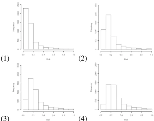
Fig. 1. Distribution of calculated (1) logit of APACHE II scoreslogit(p); and (2) probability of mortality for 4644 patients who admitted to ICU during 2000-2009.
Evaluation (APACHE) version II scoring system [11] that was routinely collected over 2000-2009 in the pilot hospital. This dataset was used to quantify patient mix in construction of baseline risks in the control charts.
The calculated logit of APACHE II scores (logit(p)) for 4644 patients led to a distribution of logit values with a mean of -2.53 and a variance of 1.05 which corresponds to an overall risk of death of 0.082 with a variance of 0.012 among patients in the pilot hospital, see Figure 1. To generate obser-vations of a process in the in-control stateyi,i= 1, ..., τ, we first randomly generated associated risks, p0i, i = 1, ..., τ, from a normal distribution (µ = −2.53, σ2 = 1.05) and
then drew binary outcomes from a Bernoulli distribution with rates of p0i, i= 1, ..., τ. Plotting the obtained observations when the associated risks are considered results in risk-adjusted control charts that are in-control.
Because we know that the process is in-control, if an out-of-control observation was generated in the simulation of the early 500 in-control observations, it was taken as a false alarm and the simulation was restarted. However, in practice a false alarm may lead to stopping the process and analyzing root causes. When no cause is found, the process would follow without adjustment.
To form an increasing linear trend in odds ratio, we then induced trends with a slope of sizes β = {0.0025,0.005,0.01,0.025,0.05,0.1} and generated obser-vations until the control charts signalled. Such drifts affects should be considered in two ways, over different base-line risk and time.
These slopes led to different shifts sizes in the in-control process rate,p0i, for theith patient after the occurrence of the change. Patients with more extreme risks of mortality are less affected compared to patients who have a probability of around 0.5.
The effect of a linear trend with a positive slope of size
β = 0.025 in odds ratio is demonstrated in Figure 2 over time, next patients say. The resultant distributions are more over-dispersed and shifted to the right and concentrates on higher values of risks in comparison with the observed risks in Figure 1-2. As seen in Figure 2-1 for the 550th
patient, when the odds ratio increases and reaches to δ1 = 2.25,
the overall risk increases to 0.15 with a variance of 0.021. This increase in the risk almost doubles after the next 150 patients, reaching to an overall risk of 0.28 with a variance of 0.033, see Figure 2-4.
To form an increasing linear trend in odds ratio, we then induced trends with a slope of sizes β = {0.0025,0.005,0.01,0.025,0.05,0.1} and generated obser-vations until the control charts signalled. We constructed
(1) (2)
(3) (4)
Fig. 2. Distribution of observable probability of mortality after (1) 50, (2) 100, (3) 150 and (4) 200 observations since occurrence of a linear trend disturbance with a slope of sizeβ= 0.025in odds ratio for 4644 patients who admitted to ICU during 2000-2009.
risk-adjusted control charts using the procedures discussed in Section II. We designed RACUSUM to detect a doubling and a halving of the odds ratio in the in-control rate, p0 =
0.082, and have an in-control average run length (ARLˆ 0)
of approximately 3000 observations. We used Monte Carlo simulation to determine decision intervals, h±
. However other approaches may be of interest; see Steiner et al. [1]. This setting led to decision intervals of h+ = 5.85 and
h− = 5.33
. As two sided charts were considered, the negative values of h−
were used. The associated CUSUM scores were also obtained through Equation (1) where yi is 0 and 1, respectively. We set the smoothing constant of RAEWMA to λ = 0.01 as the in-control rate was low and detection of small changes was desired; see Somerville et al. [9], Cook [2] and [3] for more details. The value of L was calibrated so that the same in-control average run length (ARLˆ 0) as the RACUSUM was obtained. The
resultant chart hadL= 2.83. A negative lower control limit in the RAEWMA was replaced by zero.
The linear trend disturbances and control charts were simulated in the R package (http://www.r-project.org). To obtain posterior distributions of the time and the magnitude of the changes we used the R2WinBUGS interface [12] to generate 100,000 samples through MCMC iterations in WinBUGS [13] for all change point scenarios with the first 20000 samples ignored as burn-in. We then analyzed the results using the CODA package in R [14].
V. PERFORMANCEANALYSIS
To demonstrate the achievable results of Bayesian change point detection in risk-adjusted control charts, we induced a
TABLE I
POSTERIOR ESTIMATES(MODE,SD.)OF LINEAR TREND CHANGE POINT MODEL PARAMETERS(τANDβ)FOLLOWING SIGNALS(RL)FROM
RACUSUM ((h+, h−) = (5.85,5.33))
ANDRAEWMACHARTS
(λ= 0.01ANDL= 2.83)WHEREE(p0) = 0.082ANDτ= 500. STANDARD DEVIATIONS ARE SHOWN IN PARENTHESES.
β RACUSUM RAEWMA
RL τˆ βˆ RL τˆ βˆ
(a1) (a2) (a3)
(b1) (b2) (b3)
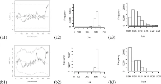
Fig. 3. Risk-adjusted (a1) CUSUM ((h+, h−) = (5.85,5.33)) and (b1) EWMA (λ = 0.01andL= 2.83) control charts and obtained posterior
distributions of (a2, b2) timeτand (a3, b3) magnitudeβof an induced linear trend with a slope of sizeβ= 0.025in odds ratio whereE(p0) = 0.082
andτ= 500.
linear trend with a slope of size β = 0.25at time τ = 500 in an in-control binary process with an overall death rate of p0 = 0.082. RACUSUM and RAEWMA, respectively,
detected an increase in the odds ratio and sinalled at the 595th
and 565th
observations, corresponding to delays of 95 and 65 observations as shown in Figure 3-a1, b1. The posterior distributions of time and magnitude of the change were then obtained using MCMC discussed in Section IV. For both control charts, the distribution of the time of the change, τ, concentrates on the values closer to 500th observation as seen in Figure 3-a2, b2. The posteriors for the magnitude of the change,β, also approximately identified the exact change size as they highly concentrate on values of less than 0.05 shown in Figure 3-a3, b3. As expected, there exist slight differences between the distributions obtained follow-ing RACUSUM and RAEWMA signals since non-identical series of binary values were used for two procedures.
Table I summarizes the obtained posteriors. If the posterior was asymmetric and skewed, the mode of the posteriors was used as an estimator for the change point model parameter (τ and β1). As shown, the Bayesian estimator of the time
outperforms chart’s signals, particularly for the RACUSUM with a delay of three observations. However, the magnitude of the slope of the linear trend tends to be over overestimated by the Bayesian estimator, obtaining 0.051 and 0.041 for RACUSUM and RAEWMA charts, respectively. Having said that, these estimates must be studied in conjunction with their corresponding standard deviations.
Applying the Bayesian framework enables us to construct probability based intervals around estimated parameters. A credible interval (CI) is a posterior probability based interval
which involves those values of highest probability in the pos-terior density of the parameter of interest. Table II presents 50% and 80% credible intervals for the estimated time and the magnitude of slope of the linear trend disturbance in odds ratio for RACUSUM and RAEWMA control charts. As expected, the CIs are affected by the dispersion and higher order behaviour of the posterior distributions. Under the same probability of 0.5 for the RACUSUM, the CI for the time of the change of size β = 0.025 in odds ratio covers 25 observations around the500thobservation whereas it increases to 35 observations for RAEWMA due to the larger standard deviation, see Table I.
As shown in Table I and discussed above, the magnitude of the changes are overestimated, however Table II indicates that the real sizes of slope are approximately contained in the respective posterior 50% and 80% CIs. Construction of probablistic intervals can be extended to other sizes of slope and direction of linear trends in odds ratio.
Having a distribution for the time of the change enables us to make other probabilistic inferences. As an example, Table III shows the probability of the occurrence of the change point in the last{25, 50, 100}observations prior to signalling in the control charts. For a linear trend with a slope of size
β = 0.025 in odds ratio, since the RACUSUM signals late (see Table I), it is unlikely that the change point occurred in the last 25 or 50 observations. In contrast, in the RAEWMA, where it signals earlier, the probability of occurrence in the last 50 observations is 0.57, then increases to 0.98 as the next 50 observations are included. These kind of probability computations and inferences can be extended to other change scenarios.
TABLE II
CREDIBLE INTERVALS FOR LINEAR TREND CHANGE POINT MODEL PARAMETERS(τANDβ)FOLLOWING SIGNALS(RL)FROMRACUSUM ((h+, h−) = (5.85,5.33))
ANDRAEWMACHARTS(λ= 0.01ANDL= 2.83)WHEREE(p0) = 0.082ANDτ= 500.
β Parameter RACUSUM RAEWMA
50% 80% 50% 80%
TABLE III
PROBABILITY OF THE OCCURRENCE OF THE CHANGE POINT IN THE LAST25, 50AND100OBSERVATIONS PRIOR TO SIGNALLING FOR
RACUSUM ((h+, h−) = (5.85,5.33))ANDRAEWMACHARTS
(λ= 0.01ANDL= 2.83)WHEREE(p0) = 0.082ANDτ= 500.
β RACUSUM RAEWMA
25 50 100 25 50 100
0.025 0.02 0.04 0.70 0.04 0.57 0.98
The above studies were based on a single sample drawn from the underlying distribution. To investigate the behavior of the Bayesian estimator over different sample datasets, for different slope sizes of β, we replicated the simula-tion method explained in Secsimula-tion IV 100 times. Simulated datasets that were obvious outliers were excluded. Table IV shows the average of the estimated parameters obtained from the replicated datasets where there exists a linear trend in odds ratio.
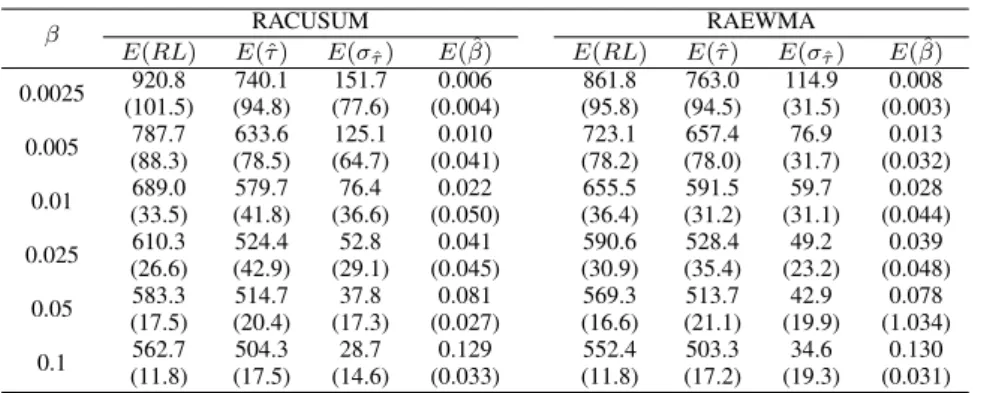
Comparison of performance of RACUSUM and RAEWMA charts in Table IV reveals that, the RAEWMA detected increasing linear trend disturbances in odds ratio faster. This superiority drops from 59 observations for
β = 0.0025to 10 observations when the slope size reaches toβ = 0.1. For a very small slope of sizeβ = 0.0025, the average of the mode,E(ˆτ), reports the740thobservation as the change point in RACUSUM, whereas the chart detected the change with a delay of 420 observations. This superiority persists for the RAEWMA chart, however a delay of 263 observations is still associated with the estimate of the time,
τ, for β= 0.0025following RAEWMA signal.
Table IV shows that, although the RACUSUM signals later than the alternative, RAEWMA, particularly over small to medium slope sizes, the average of posterior estimates for the time, E(ˆτ), outperforms the estimates obtained for RAEWMA charts. A less delay of 23 observations is ob-tained forβ = 0.0025scenario. This delay drops when the slop size increases. Over medium to large sizes of slope,β= {0.025,0.05,0.1}, the bias of the Bayesian estimator,E(ˆτ), did not exceed 24 observations for the RACUSUM. This bias slightly increased for the RAEWMA chart, reaching to 28 observations, yet significantly outperformed the chart’s signal. At best, the RACUSUM and RAEWMA signals at the 562nd
and 552nd
observations for the most extreme jump in the slope of the linear trend in odds ratio were also outperformed by posterior modes,E(ˆτ), that exhibited a bias
of four and three observations, respectively.
Table IV indicates that in both risk-adjusted control charts, the variation of the Bayesian estimates for time tends to reduce when the magnitude of slope increases. The mean of the standard deviation of the posterior estimates of time,
E(στˆ), also decreases when the slope sizes increases. The
average of the Bayesian estimates of the magnitude of the change,E( ˆβ), shows that the posterior modes tend to over-estimate slope sizes. As seen in Table IV, better over-estimates are obtained in moderate to large slopes. Having said that, Bayesian estimates of the magnitude of the change must be studied in conjunction with their corresponding standard deviations. In this manner, analysis of credible intervals is effective.
VI. COMPARISON OFBAYESIANESTIMATOR WITH
OTHERMETHODS
To study the performance of the proposed Bayesian esti-mators in comparison with those introduced in Section I, we ran the available alternatives, built-in estimators of Bernoulli EWMA and CUSUM charts, within the replications dis-cussed in Section V. Based on Page [4] suggestion, if an increase in a process rate detected by CUSUM charts, an estimate of the change point is obtained through ˆτcusum =
max{i : Xi+ = 0}. We modified the built-in estimator of EWMA proposed by Nishina [6] and estimated the change point usingτˆewma=max{i:Zoi≤Zpi} following signals of an increase in the Bernoulli rate.
Table V shows the average of the Bayesian estimates,
τb, and detected change points provided by the built-in estimators of CUSUM,τcusum, and EWMA,τewma, charts for drifts in the odds ratio, OR. The built-in estimators of EWMA and CUSUM charts outperform associated signals over all drifts in the odds ratio, however they tend to under-estimate the exact change point when the magnitude of slope is large, β = 0.1. The CUSUM built-in estimator, ˆτcusum, outperforms the alternative built-in estimator over small to moderate slopes, exactly over the same range of changes in which the Bayesian estimates obtained for RACUSUM are superior.
The Bayesian estimator,τˆb, is outperformed by both built-in estimators, ˆτcusum and τˆewma, with less delays which is at most 35 observations obtained for RAEWMA for
β = 0.005. Having said that, considering corresponding
TABLE IV
AVERAGE OF POSTERIOR ESTIMATES(MODE,SD.)OF LINEAR TREND CHANGE POINT MODEL PARAMETERS(τANDβ)FOR A DRIFT IN ODDS RATIO FOLLOWING SIGNALS(RL)FROMRACUSUM ((h+, h−) = (5.85,5.33))
ANDRAEWMACHARTS(λ= 0.01ANDL= 2.83)WHERE
E(p0) = 0.082ANDτ= 500. STANDARD DEVIATIONS ARE SHOWN IN PARENTHESES.
β RACUSUM RAEWMA
E(RL) E(ˆτ) E(στˆ) E( ˆβ) E(RL) E(ˆτ) E(στˆ) E( ˆβ)
0.0025 920.8 740.1 151.7 0.006 861.8 763.0 114.9 0.008 (101.5) (94.8) (77.6) (0.004) (95.8) (94.5) (31.5) (0.003)
0.005 (88.3)787.7 (78.5)633.6 (64.7)125.1 (0.041)0.010 (78.2)723.1 (78.0)657.4 (31.7)76.9 (0.032)0.013
0.01 (33.5)689.0 (41.8)579.7 (36.6)76.4 (0.050)0.022 (36.4)655.5 (31.2)591.5 (31.1)59.7 (0.044)0.028
0.025 (26.6)610.3 (42.9)524.4 (29.1)52.8 (0.045)0.041 (30.9)590.6 (35.4)528.4 (23.2)49.2 (0.048)0.039
0.05 583.3 514.7 37.8 0.081 569.3 513.7 42.9 0.078 (17.5) (20.4) (17.3) (0.027) (16.6) (21.1) (19.9) (1.034)
TABLE V
AVERAGE OF DETECTED TIME OF A LINEAR TREND CHANGE IN ODDS RATIO OBTAINED BY THEBAYESIAN ESTIMATOR(τb), CUSUMANDEWMA
BUILT-IN ESTIMATORS FOLLOWING SIGNALS(RL)FROMRACUSUM ((h+, h−
) = (5.85,5.33))ANDRAEWMACHARTS(λ= 0.01AND
L= 2.83)WHEREE(p0) = 0.082ANDτ= 500. STANDARD DEVIATIONS ARE SHOWN IN PARENTHESES.
β RACUSUM RAEWMA
E(RL) E(ˆτcusum) E(ˆτb) E(RL) E(ˆτewma) E(ˆτb) 0.0025 920.8 727.7 740.1 861.8 739.4 763.0 (101.5) (131.9) (94.8) (95.8) (128.5) (94.5)
0.005 787.7 605.8 633.6 723.1 622.3 657.4 (88.3) (110.2) (78.5) (78.2) (103.9) (78.0)
0.01 (33.5)689.0 (56.2)559.7 (41.8)579.7 (36.4)655.5 (55.5)573.2 (31.2)591.5
0.025 (26.6)610.3 (62.6)513.1 (42.9)524.4 (30.9)590.6 (67.6)514.0 (35.4)528.4
0.05 (17.5)583.3 (56.5)495.2 (20.4)514.7 (16.6)569.3 (61.4)506.1 (21.1)513.7
0.1 562.7 483.4 504.3 552.4 497.8 503.3 (11.8) (45.7) (17.5) (11.8) (63.2) (17.2)
standard deviations over replications, the Bayesian estimator remains a reasonable alternative. The superiority of the built-in estimators drops when slope size built-increases sbuilt-ince they tend to underestimate the time of the change, whereas the average of posterior modes estimates more accurately. Comparison of variation of estimated change points also supports the superiority of the Bayesian estimators over alternatives across linear trend with a small slope.
VII. CONCLUSION
In this paper, using a Bayesian framework, we modeled change point detection for a clinical process with dichoto-mous outcomes, death and survival, where patient mix was present. We considered an increasing drift in odds ratio, caused by a linear trend with a positive slope, of the in-control rate. We constructed Bayesian hierarchical models and derived posterior distributions for change point estimates using MCMC. The performance of the Bayesian estimators were investigated through simulation when they were used in conjunction with well-known risk-adjusted CUSUM and EWMA control charts monitoring mortality rate in the ICU of the pilot hospital where risk of death was evaluated by APACHE II, a logistic prediction model. The results showed that the Bayesian estimates significantly outperform the RACUSUM and RAEWMA control charts in change detection over different scenarios of magnitude of slopes in drifts. We then compared the Bayesian estimator with built-in estimators of EWMA and CUSUM. Although the Bayesian estimator outperformed by the built-in estimators, they re-main viable alternative when precision of the estimators are taken into account.
Apart from accuracy and precision criteria used for the comparison study, the posterior distributions for the time and the magnitude of a change enable us to construct probabilistic intervals around estimates and probabilistic inferences about the location of the change point. This is a significant ad-vantage of the proposed Bayesian approach. Furthermore, flexibility of Bayesian hierarchical models, ease of extension to more complicated change scenarios such as decreasing lin-ear trends, nonlinlin-ear trends, relief of analytic calculation of likelihood function, particularly for non-tractable likelihood functions and ease of coding with available packages should be considered as additional benefits of the proposed Bayesian change point model for monitoring purposes.
The investigation conducted in this study was based on a specific in-control rate of mortality observed in the pilot hos-pital. Although it is expected that superiority of the proposed Bayesian estimator persists over other processes in which the in-control rate and the distribution of baseline risk may differ, the results obtained for estimators and control charts over various change scenarios motivates replication of the study using other patient mix profiles. Moreover modification of change point model elements such as replacing priors with more informative alternatives, or truncation of prior distributions based on type of signals and prior knowledge, may be of interest.
REFERENCES
[1] Steiner, S.H., Cook, R.J., Farewell, V.T., & Treasure, T., “Monitoring surgical performance using risk-adjusted cumulative sum charts”,
Biostatistics, V1, N4, pp. 441-452, 2000.
[2] Cook, D., “The Development of Risk Adjusted Control Charts and Machine learning Models to monitor the Mortality of Intensive Care Unit Patients”,Ph.D. Thesis; University of Queensland, 2004. [3] Grigg, O.V. & Spiegelhalter, D.J., “A Simple Risk-Adjusted
Exponen-tially Weighted Moving Average”,Journal of the American Statistical Association, V102, N477, pp. 140-152, 2007.
[4] Page, E., “Continuous inspection schemes”.Biometrika, V41, N1/2, pp. 100-115, 1954.
[5] Page, E., Cumulative sum charts. Technometrics, V3, N1, pp. 1-9, 1961.
[6] Nishina, K., “A comparison of control charts from the viewpoint of change-point estimation”,Quality and Reliability Engineering Inter-national, V8, pp. 537-537, 1992.
[7] Gelman, A., Carlin, J., Stern, H. & Rubin, D.,Bayesian data analysis: Chapman&Hall/CRC, 2004.
[8] Cook, D.A., Duke, G., Hart, G.K., Pilcher, D., Mullany, D., “Review of the Application of Risk-Adjusted Charts to Analyse Mortality Outcomes in Critical Care”, Critical Care Resuscitation, V10, N3, pp. 239-251, 2008.
[9] Somerville, S.E., Montgomery, D.C. & Runger, G.C., “Filtering and smoothing methods for mixed particle count distributions”, journal International Journal of Production Research, V40, N13, pp. 2991-3013, 2002.
[10] Montgomery D.C.,Introduction to Statistical Quality Control(Sixth ed.): Wiley, 2008.
[11] Knaus, W., Draper, E., Wagner, D.,& Zimmerman, J. (1985). APACHE II: a severity of disease classification system.Critical care medicine,
13(10), 818-829.
[12] Sturtz, S., Ligges, U., & Gelman, A., “R2WinBUGS: A package for running WinBUGS from R”,Journal of Statistical Software, V12, N3, pp. 1-16, 2005.