Printed version ISSN 0001-3765 / Online version ISSN 1678-2690
www.scielo.br/aabc
Use of convolution and geotechnical rock properties to analyze free flowing discharge test
EDSON WENDLAND1, LUIS HENRIQUE GOMES2 and RODRIGO M. PORTO1 1
Universidade de São Paulo, Departamento de Hidráulica e Saneamento, Caixa Postal 359, 13560-970 São Carlos, SP, Brasil
2Departamento de água e Energia Elétrica, Av. Otávio Pinto Cesar, 1400, Cid. Nova, 15085-360 São José do Rio Preto, SP, Brasil
Manuscript received on November 6, 2012; accepted for publication on April 15, 2013
ABSTRACT
Discharge tests are conducted in order to determine aquifers transmissivity (T) and storage coefficient (S). However the interpretation of test data is not unique and the results may vary depending on adopted hypothesis. In this work, the convolution technique is applied for the reconstruction of observed drawdown
curves aiming for the reduction of uncertainty. The interference between a flowing well and an observation well is evaluated in order to determine the hydrogeological parameters of the confined Guarani Aquifer
System (Araujo et al. 1999). Discharge test data are analyzed according to the Jacob and Lohman (1952) method. The application of convolution enabled the determination of the most reliable solution. Obtained transmissivity (T = 411.0 m2/d) and storage coefficient (S = 2.75x10⁻⁴) are close to values estimated by direct evaluation of the geotechnical sandstone properties.
Key words: hydrogeology, groundwater, transmissivity, storage coefficient, pumping test.
Correspondence to: Edson Wendland E-mail: [email protected]
INTRODUCTION
The determination of aquifers transmissivity (T) and storage coefficient (S) is based on the observation of aquifer’s response to a given stimulation. In order to characterize hydrogeological systems, discharge tests are conducted. The present work explores the use of convolution (Barlow et al. 2000, Ostendorf et al. 2007, Olsthoorn 2008) to a discharge test performed in an artesian aquifer.
The interpretation of discharge tests data relies on the physical conditions of the aquifer (e.g. unconfined, confined, leaky, homogeneous, isotropic), the drawdown regime (steady or transient), pumping condition
(constant or variable discharge), the hydraulic boundaries, and the well construction (fully or partially penetrating). In this sense, many authors (overview given by Freeze and Cherry 1979) have provided
mathematical approaches for data analyses according to the different pumping conditions. Artesian confined aquifers, however, do not need pumping energy, and water from the aquifer flows naturally at the well head.
The analysis of this problem was described originally by Jacob and Lohman (1952).
Due to missing observation wells, some discharge tests interpretation are based only on transient drawdown data obtained from the pumping well itself. Although this situation is undesirable it is necessary, since the
confined aquifer is quite deep (up to 1200m) and drilling observation wells is economically unviable. Since the
solution is not unique, a wide spreading of values is expected and the reliability of the obtained parameters is
quite uncertain. As a consequence, the transmissivity and storage coefficient obtained from pumping tests vary
substantially even for homogeneous aquifers. For the Guarani Aquifer System (Araujo et al. 1999), for instance, available transmissivity values may vary between 150 m2/d (Borghetti et al. 2004) and 1000 m2/d (Sinelli and Gallo 1980), while storage coefficients range from 10-3 (DAEE 1974) to 10-6 (Borghetti et al. 2004). However, this apparent strong heterogeneity results mainly from the unreliable interpretation of the discharge tests.
In the present work, the interference between a 1244 m deep flowing well and an observation well is evaluated in order to determine the hydrogeological parameters of the confined Guarani Aquifer System.
Discharge test data are analyzed according to the Jacob and Lohman (1952) method. The convolution technique is applied for the reconstruction of observed drawdown curves aiming for the reduction of uncertainty. The obtained hydrogeological parameters are further evaluated by estimate of the storage
coefficient based on direct evaluation of geotechnical properties.
MATERIALS AND METHODS
CONCEPTUAL MODEL
The discharge test in a flowing well is a classic test known in Literature as the Constant Drawdown Problem,
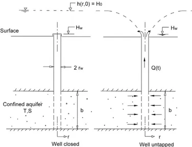
described initially by Jacob and Lohman (1952). The conceptual model is presented schema tically in Figure 1 (theoretical problem).
A well with a finite radius rW is drilled through an infinite confined aquifer with thickness b, hydraulic transmissivity T and storage coefficient S. The aquifer is artesian and the well has remained closed for a long period of time.
At a given instant t=0, the hydraulic head (poten tiometric surface) in the aquifer is H0. At instant t=0+, the well is opened and the hydraulic head drops immediately to HW, which corresponds to the well head. Since the aquifer is artesian, water begins to flow naturally. In the absence of an external source (recharge), the well will keep flowing until the hydraulic head in the whole aquifer is reduced to HW.
THE MATHEMATICAL MODEL FOR FLOWING WELLS
The radial flux to a flowing well in a confined, homogeneous and isotropic aquifer can be described by the flow equation
S @h
@t = T @2h @r2 +
1
r
@h
@r , (1)
where t is the time since the test began, r is the radial distance from the well center, S is the storage coefficient and T represents the aquifer transmissivity.
According to Jacob and Lohman (1952), the solution for equation (1) is given as
Q = 2πT swG(α), (2)
where Q is the flowing discharge rate. The type function and the variable α are defined as
G(α) = 4α
π
∞
∫
0
x e-ax2[π 2 +tan
-1Y0(x)
J0(x) ]
dx , α = Tt (3)
Srw2
where J0(x) and Y0(x) are zero order Bessel functions of the first and second types, respectively. As shown
by Lohman (1972), G(α) can be approximated by 2/W(u), where u = Srw 2
4Tt is the classical dimensionless
time parameter.
Following a methodology similar to the Cooper and Jacob (1946) method, the aquifer transmissivity T and storage coefficient S may be determined from a semi-logarithmic graph constructed with observed data. The same problem was analyzed by Peng et al. (2002), following a solution proposed by Carslaw and Jaeger (1939), which was based on the application of the Laplace Transform and the Boundary Integral Method. An alternative approach was also proposed by Ojha (2004). Wendland (2008) presented a correction for head losses due to friction in the well casing.
CONVOLUTION
In order to verify the validity of the hydrogeological parameters obtained from the interpretation of the
discharge test data, the drawdown curves observed in flowing and observation wells can be reconstructed
by convolution.
Convolution (Olsthoorn 2008) is a form of mathematical superposition. In general, the superposition principle is used to evaluate the temporal behavior of a given variable due to different effects, which can be summed. Convolution is used to evaluate in a certain instant (t*), the superposition of time variable effects. Convolution is based on the response of a system, caused by an impulse or excitation, to simulate the effect of variable strengths in space and time. The application of convolution can be limited, if the necessary information (data) about impulses in the past are not available. However the lack of data is a limitation to any analysis technique and is not restricted to convolution.
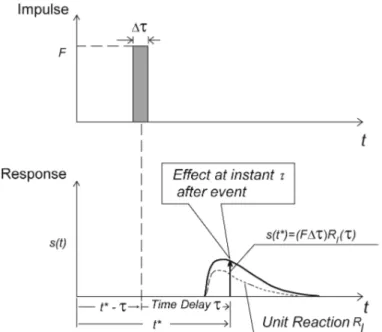
Figure 2 presents a unit response (RI). It is defined for an infinitesimal impulse with unit intensity
∆τ lim (→0 F ∆τ) RI (τ) = 1.
In case of a sequence of impulses, each one has its own response, displaced in time. The final system
response (s) in a given instant (t*) results from the summation of individual responses:
s(t*) = ∞Σ
i=0[F(t*‒ τi) ∆τi] RI (τi). (4)
When ∆τ → 0, the summation transforms into a Duhamel (1797 to 1872) convolution integral, continuous in time
s(t*) = ∫ t=0 ∞
F(t*‒ τ) RI (τ)dτ. (5)
According to equations 4 and 5, to obtain the system response (s) in a given instant (t*), the impulses
(or effects) in previous instants (τ), i.e., F(t*‒ τ), must be multiplied by the corresponding unit responses (RI (τ)) and summed up (integrated).
The time interval ∆τi = τi‒ τi ‒1can be variable. It is not necessary to be constant during a convolution.
TEST CASE
The described methodology was applied to a flowing and an observation well drilled 832m apart with diameters of 0.11 and 0.20m, respectively, in the confined Guarani Aquifer System. Pressure in both well
heads was monitored with manometers during the discharge test. The discharge (Q) and the corresponding drawdown (sw) and (so) registered at the flowing and observation wells, respectively, are presented in Table I. In this data, head losses in the flowing well have been considered as discussed by Wendland (2008).
Theoretically, a constant drawdown and variable discharge at the flowing well is expected.
However, as shown in Table I, the drawdown observed in the flowing well increases 2.32m (from 11.98m
Figure 2 - The unit response (dashed line) is the system response to a unitary impulse,
∆τ lim (→0 F ∆τ) RI (τ) = 1. The system response s(t*)
t (min)
Q (m3/h)
sw (m)
so (m)
1 179.44 11.98 0.0
2 175.19 12.75 0.0
3 174.41 12.70 0.0
4 174.01 12.72 0.0
5 174.01 12.62 0.0
6 174.21 12.71 0.0
7 174.21 12.61 0.0
8 174.80 12.57 0.0
9 174.99 12.56 0.0
10 175.39 12.53 0.0
12 175.58 12.47 0.0
14 175.58 12.52 0.0
16 175.58 12.47 0.0
18 175.19 12.65 0.0
20 174.80 12.52 0.0
25 174.01 12.62 0.0
30 173.22 12.62 0.0
35 172.43 12.72 0.0
40 172.03 12.64 0.0
50 171.04 12.71 0.0
60 170.03 12.87 0.1
70 169.63 12.79 0.1
80 169.02 13.13 0.0
90 168.41 13.07 0.1
100 168.00 13.19 0.2
120 166.78 13.26 0.2
150 166.16 13.30 0.2
180 165.33 13.35 0.3
210 164.71 13.44 0.3
240 164.08 13.48 0.3
270 163.46 13.51 0.3
300 163.25 13.53 0.5
330 162.83 13.55 0.5
360 162.62 13.56 0.5
390 162.19 13.59 0.6
420 161.98 13.60 0.6
480 161.56 13.62 0.7
540 161.14 13.70 0.7
600 160.92 13.71 0.8
660 160.71 13.82 0.8
720 160.50 13.94 0.7
780 160.28 13.95 0.7
840 160.28 13.95 0.7
900 160.07 13.96 0.7
960 159.64 13.99 0.7
1020 159.21 14.01 0.7
TABLE I
to 14.30m) during the 34 hour-long discharge test. This occurs due to depressurization of the confined
aquifer. As a consequence, both drawdown and discharge vary and the assumptions of Theis (1935) and Jacob and Lohman (1952) interpretation methods are not respected.
Nevertheless, the reliability of the hydrogeological parameters obtained from test data interpretation can be increased. The varying discharge observed, is considered an impulse and the drawdown is calculated by applying the convolution technique as
s(t*) = ∫ t=0 ∞
Q(t*‒ τ) RI (τ)dτ. (6)
where the unit response is given by Theis function
RI (τ) = @RD (τ)
@τ = 1 4πT
e‒u
τ (7)
RESULTS AND DISCUSSION
The mathematical model for flowing wells was utilized to determine the aquifer transmissivity and storage coefficient following the Jacob and Lohman linear fitting approach. Ignoring the data registered
in the first 12 min (case 1), the observed values are fitted by a straight line given by equation sw/Q = 15.982 ln(t/rw2) + 100.75, with a correlation factor of R2 = 0.9893, as shown in Figure 3. On this graphic, variable Q, as given in Table I, was used for the sw/Q axis. Mathematically the proposed fit does not lead to zero drawdown at zero time because the first 12 min of data have been ignored in the adjustment. For this period the fit is not valid. The calculated transmissivity and storage coefficient are T = 430 m2/d and S = 2.0x10⁻⁵, respectively. The Jacob and Lohman approach is valid for u<0.03. Considering the obtained results (S and T), the approach is consequently valid for t > 0.0037 s.
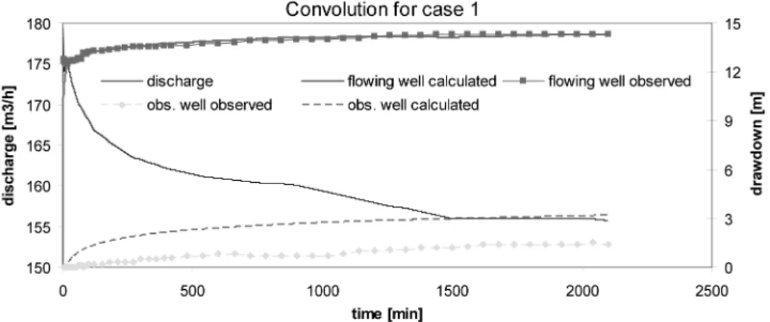
The obtained hydrogeological parameters were used to reconstruct the drawdown curves applying
convolution to both flowing and observation wells. The time interval for convolution was chosen as constant
with ∆τ = 1 min. Figure 4 shows a comparison between calculated and observed drawdown curves, as given in Table I.
t (min)
Q (m3/h)
sw (m)
so (m)
1080 158.78 14.04 0.8
1140 158.35 14.06 1.0
1200 157.91 14.19 1.0
1260 157.48 14.21 1.1
1320 157.26 14.22 1.1
1380 156.83 14.25 1.2
1440 156.39 14.27 1.2
1500 155.95 14.30 1.2
1560 155.95 14.30 1.3
1620 155.95 14.30 1.4
1980 155.95 14.30 1.4
2040 155.95 14.30 1.5
Figure 3 - Diagram of sw/Q x t/rw
2for the flowing well, ignoring the first 12 min of test data (case 1).
Figure 4 - Comparison between the calculated and observed drawdown curves for flowing and observation wells, using parameters from the first analysis (case 1).
As shown in Figure 4, calculated and observed drawdown for the flowing well agree very well, indicating that the transmissivity and storage coefficient values obtained in Figure 3 are acceptable for confined sandstone aquifers. However, calculated and observed drawdown for the observation well fully
diverges. The calculated drawdown is larger than the observed data, indicating that the estimated storage
coefficient is too small.
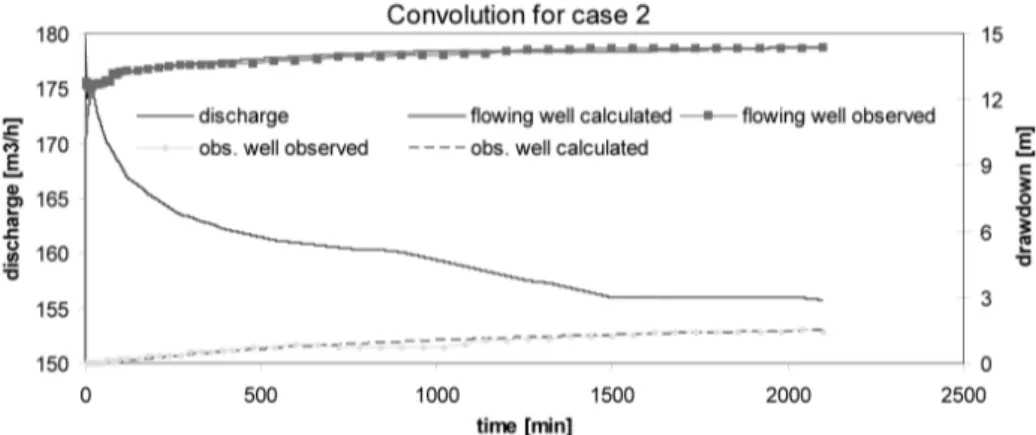
A new interpretation of test data for the flowing well (sw) is shown in Figure 5. In this case (2), data registered in the first 25 min were ignored. The observed values are fitted by a straight line given by equation sw/Q = 16.724 ln(t/rw2) + 61.217, with a correlation factor of R2 = 0.9899. The new calculated transmissivity and storage coefficient are T = 411 m2/d and S = 2.75x10⁻⁴, respectively.
Again the obtained hydrogeological parameters were used to reconstruct the drawdown curves applying convolution. Figure 6 shows a comparison between calculated and observed drawdown curves for both
As shown in Figure 6, calculated and observed drawdown for both flowing and observation wells agree very well. Transmissivity and storage coefficient values obtained in Figure 5 are able to adequately
reproduce the hydraulic head variation in both wells during the discharge test.
The comparison between results obtained in the first and second analysis indicates that hydrogeologic
parameters obtained from single well pumping tests should be used carefully, since the interpretation of test data is not unique. Although the aquifer transmissivity (T) appears to be almost the same in both cases (430 and 411 m2/d, respectively), the difference in the storage coefficient (S) is of almost one order of magnitude (2.0x10⁻⁵ and 2.8x10⁻⁴, respectively). Convolution applied to reconstruct the observed drawdown curves proved to be a powerful tool for result evaluation.
In order to further verify the interpretation of test data, the storage coefficient was estimated from the physical properties of the aquifer. According to Fetter (2001), the specific storage coefficient (So, [m-1]) can be determined from the relation
So = γw[nβ + (1 ‒ n)α] (6)
Figure 5 - Diagram of sw/Q x t/rw
2for the flowing well, ignoring the first 25 min of test data (case 2).
in which γw is the fluid specific weight (9810 N/m3), n is the aquifer porosity (-), β is the fluid compressibility (4.6x10⁻¹⁰ m2/N) and αis the porous medium compressibility (m2/N).
Porous medium compressibility (7.81x10⁻¹¹ m2/N) and porosity (19.2%) for the Botucatu Sandstone, which compounds the Guarani Aquifer System, were determined by laboratory measurements (Bortolucci
2009). Substituting these values in equation (6) leads to a specific storage coefficient So = 1.43x10⁻⁶ m-1. The theoretical storage coefficient (St [-]) is obtained by multiplying So by the aquifer thickness (b [m])
St = So b (7)
Given the mean thickness of 200m for the Guarani Aquifer System in the well (Wendland 2008), the
theoretical storage coefficient is estimated as St = 2.86x10⁻⁴. This value is very close to the value obtained in the interpretation of discharge test data S = 2.75x10⁻⁴, proving its coherence.
The mean hydraulic conductivity (K) for the Guarani Aquifer System in the study area can be determined from the relation T = Kb. Considering the transmissivity T = 411 m2/d determined in the discharge test, the hydraulic conductivity is K = 2.06 m/d = 2.38x10⁻⁵ m/s. This value agrees with results presented in Literature (Gastmans and kiang 2005).
CONCLUSIONS
This paper presented the evaluation of discharge test data obtained in a flowing and in an observation well.
Discharge test data were analyzed according to the Jacob and Lohman method in order to determine the
hydrogeological parameters of the confined Guarani Aquifer System. Since the solution is not unique, two situations were considered leading to different values of transmissivity and storage coefficient.
The convolution technique was applied to reconstruct observed drawdown curves reducing the uncertainty about obtained results. The application of convolution allowed for the determination of transmissivity (T = 411 m2/d) and storage coefficient (S = 2.75x10⁻⁴), which appear to be representative of the confined Guarani Aquifer in the study area. Convolution proved to be a powerful tool for result
validation and reliability assurance.
In order to further verify the interpretation of test data, the storage coefficient was estimated from
the geotechnical properties of the aquifer. The obtained result is very close to the value determined by convolution, proving its coherence.
The results obtained in this work indicate that some hydrogeological parameters available in Literature should be carefully used, since inadequate interpretation of pumping test data may lead to unreliable values. On the other hand, applying different complementary techniques to determine the parameters improves the
confidence of the obtained results.
ACKNOWLEDGMENTS
The development of this work was partially supported by Conselho Nacional de Desenvolvimento Científico e
Tecnológico (CNPq/Brazil, fellowship).
RESUMO
hipóteses adotadas. Neste trabalho, a técnica de convolução é aplicada para a reconstrução de curvas de rebaixamento observadas, objetivando a redução de incertezas. A interferência entre um poço jorrante e um poço de observação é
avaliada para determinar os parâmetros hidrogeológicos do Sistema Aquífero Guarani confinado (Araujo et al. 1999).
Os dados do teste de descarga são analisados de acordo com o método de Jacob e Lohman (1952). A aplicação da
convolução permitiu a determinação da solução mais confiável. A transmissividade (T = 411.0 m2/d) e o coeficiente
armazenamento (S = 2.75x10⁻⁴) obtidos estão próximos de valores estimados através da avaliação direta das propriedades geotécnicas do arenito.
Palavras-chave: hidrogeologia, água subterrânea, transmissividade, coeficiente de armazenamanto, teste de bombeamento.
REFERENCES
ARAúJO LM, FRANçA AB AND POTER PE. 1999. Hydrogeology of the Mercosul Aquifer System in the Paraná and Chaco-Paraná Basins, South America, and comparison with the Navajo-Nugget Aquifer System, USA. Hydrogeol J 7: 317-336.
BARLOW PM, DESIMONE LA AND MOENCH AF. 2000. Aquifer response to stream-stage and recharge variations. II. Convolution method and applications. J Hydrol 230: 211-229.
BORGHETTI NRB, BORGHETTI JRE AND ROSA FILHO EF. 2004. Aquífero Guarani – A verdadeira integração dos países do MERCOSUL, Rio de Janeiro: Fundação Roberto Marinho, 214 p.
BORTOLUCCI AA. 2009. Geotechnical parameters for the Botucatu Sandstone determined by laboratory measurements (personal communication).
CARSLAW HS AND JAEGER JC. 1939. Some two-dimensional problems in conduction of heat with circular symmetry. Heat Conduction 46: 361-388.
COOPER HH AND JACOB CE. 1946. A generalized graphical method for evaluating formation constants and summarizing well field
history. Am Geophys Union Trans 27: 526-534.
DAEE - DEPARTAMENTO DE áGUAS E ENERGIA ELéTRICA. 1974. Estudo de águas subterrâneas – Região Administrativa 6 - Ribeirão
Preto, São Paulo: DAEE Departamento de águas e Energia Elétrica, v.4. FETTER CW. 2001. Applied Hydrogeology. New Jersey: Prentice Hall, 4th ed., 598 p. FREEzE RA AND CHERRy JA. 1979. Groundwater. Englewood Cliffs, NJ, Prentice-Hall, 604 p.
GASTMANS D AND kIANG CH. 2005. Avaliação da hidrogeologia e hidroquímica do Sistema Aqüífero Guarani (SAG) no estado de
Mato Grosso do Sul. Águas Subterrâneas 19(1): 35-48.
JACOB CE AND LOHMAN SW. 1952. Nonsteady flow to a well of constant drawdown in an extensive aquifer. Trans Am Geophys
Union 33(4): 559-569.
LOHMAN SW. 1972. Ground-Water hydraulics. Geological Survey Professional Paper, 708, Washington: United States Government Printing Office.
OJHA CSP. 2004. Aquifer parameters estimation using artesian well test data. Journal of Hydrologic Engineering 9(1): 64-67. OLSTHOORN TN. 2008. Do a bit more with convolution. Ground Water 46(1): 13-22. doi:10.1111/j.1745-6584.2007.00342.x OSTENDORF DW, DEGROOT DJ AND HINLEIN ES. 2007. Unconfined aquifer response to infiltration basins and shallow pump tests.
J Hydrol 338: 132-144. doi:10.1016/j.jhydrol.2007.02.033
PENG Hy, yEH HD AND yANG Sy. 2002. Improved numerical evaluation of the radial groundwater flow equation, Advances in
Water Resources 25(6): 663-675.
SINELLI O AND GALLO G. 1980. Estudo hidroquímico e isotópico das águas subterrâneas na região de Ribeirão Preto, SP. Rev Bras
Geocienc 10: 129-140.
THEIS CV. 1935. The relation between the lowering of the piezometric surface and the rate and duration of discharge of a well using groundwater storage. Trans Am Geophysical Union 16: 519-524.