Farid Majana,
Walter Mascarenhas,
Martin Tygel,
Lúcio T. Santos
Recebido em 16 dez. 2003 / Aceito em 28 maio 2004Received dec. 16, 2003 / Accepted may 28, 2004
ABSTRACT
The Common Reflection Surface (CRS) method is a powerful extension of the well established Common Midpoint (CMP) method in the sense that it is able to accept, at each trace location on the zero-offset (ZO) section to be constructed, reflection data from source and receiver pairs that are arbitrarily located around that point. The CRS method uses the general hyperbolic moveout, that depends, in the 2D situation considered in this work, on three parameters. One of these parameters is the classical NMO velocity. As in the single-parameter CMP method, the CRS parameters or attributes are estimated by a direct application of suitable coherence analysis to the input multicoverage data. The estimation of the three CRS parameters is generally performed in two steps. The first step has a global character and aims in obtaining an initial estimate of the parameters. The second step has a local character, trying to refine the previous initial values to more accurate values. Here we focus on the refinement step assuming that initial estimates have been already provided. We review and compare three of these methods and compare their performances on illustrative synthetic and real data examples. Comparisons with the application of the conventional CMP method are also provided. Keywords: CRS, Optimization, Stacking
RESUMO
O método da superfície comum de reflexão CRS (Common Reflection Surface) é uma extensão do tradicional método NMO (Normal Move Out). O CRS permite somar ou empilhar traços dispostos em configurações mais gerais que as de ponto médio comum CMP (Common MidPoint). Para tal propósito, o método CRS utiliza uma equação de tempo de trânsito generalizada, que depende da tradicional velocidade NMO e de outros parâmetros. Da mesma maneira que no método NMO, os parâmetros CRS são determinados a partir de uma análise de coerência nos dados de cobertura múltipla. A construção das seções simuladas de afastamento nulo requer três parâmetros no caso 2D. Este trabalho trata a estimação destes parâmetros e compara três algoritmos de otimização local aplicados ao refinamento dos parâmetros CRS. As comparações são feitas usando dados sintéticos e reais.
Palavras-chave: CRS, otimização, empilhamento
1 NUMERICA LTDA - Cll 46 # 33-18 Of. 302 - Bucaramanga - Santander - Colombia - Teléfono +57 (7) 657 6894 TeleFax: +57 (7) 643 6501 - e-mail: [email protected] 2 Instituto de Matemática e Estatística da Universidade de São Paulo (IME-USP) - Rua do Matão, 1010 - Cidade Universitária - CEP 05508-090 - São Paulo - SP - Telefone: +55 11 3091-5411
- Fax: +55 11 3814-4135 - e-mail: [email protected]
3 UNICAMP – IMECC - Praça Sergio Buarque de Holanda, 651 - Cidade Universitária - Barão Geraldo - Caixa Postal: 6065 - Campinas - São Paulo - 13083-859 - e-mail: [email protected] 4 Departamento de Matemática Aplicada - IMECC - UNICAMP - Caixa Postal 6065 - 13081-970 Campinas (SP) - Fax. (19) 3289-5766 - Tel. (19) 3788-5975 - e-mail: [email protected]
INTRODUCTION
This work discusses the estimation of the Common Reflection Surface (CRS) parameters for seismic imaging in the 2D situation. More specifically, we assume that sources and receivers are located on a sin-gle seismic line, for simplicity supposed to be horizontal and, moreover, that propagation occurs on the vertical plane below the seismic line. A final assumption is that of a known, locally constant near-surface veloci-ty at each central point. This means that, at each central point, x0, the medium velocity, v0 is supposed to have negligible gradients. Note, however, that the velocities, v0may vary for varying central points, x0. As the classical CMP method, the CRS method leads to simulated zero-offset (ZO) sections for points of interest along the seismic line. As usual practice, we consider that the traces of the ZO section to be simulated are located at given CMPs. Each ZO trace location, called a central point, is specified by its (midpoint) coordinate, x0, along the seismic line. Both methods, CMP and CRS, gives rise to a simulated ZO trace at x0, by stacking the data at each time sample t0.
In the CMP method, the stacked value corresponding to (x0, t0)
is obtained taking into account only the traces in the CMP gather that refer to x0. The stack is performed according to the NMO traveltime formula t h t h v NMO 2 02 2 2 4 ( )= + , (1)
where h is the half-offset of the source-receiver pair under consideration and vNMO is the NMO-velocity associated to the point (x0, t0). The
parameter vNMOis estimated applying a coherence (e.g., semblance) analysis to the CMP gather related to x0. The procedure is generally known as velocity analysis and is performed for a few user-selected time samples only. These correspond to key reflection events that are ma-nually picked by the interpreter. The NMO-velocity values at the re-maining time samples are obtained by simple interpolation, yielding the
vNMO values for the whole ZO trace at x0.
The CMP method has well-known advantages: enhancement of signal-to-noise ratio, attenuation of undesirable events and a quick and efficient implementation. However, it has two drawbacks: the coherency analysis is restricted to CMP gathers, which encompass only part of the available data and the need to manually pick the data on selected events. The CRS method, although computationally more expensive, does not have such drawbacks and preserves the good features of the CMP method. It applies the general hyperbolic traveltime moveout given by
t x h2 t0 A x x0 B x x Ch 2 0 2 2 , ( )= + ( − ) + ( − ) + (2)
for all source receivers in an appropriate neighborhood of the central point, x0. In the above formula, x denotes the midpoint and half-offset coordinates of the source receiver pair for which the traveltime is com-puted. As a result, the CRS method makes a better use of the available data, because such neighborhoods contain significantly more traces than the CMP gather. Moreover, the CRS method is fully automatic and does not depend on the manual specification of NMO velocities.
The 2D hyperbolic traveltime moveout (2) depends on three pa-rameters, as opposed to the single vNMOparameter in equation (1). It is convenient to write these three parameters as
A v B v PST =2 = 4 0 2 sin , , β and C v NMO = 42 , (3)
whereβ is the angle between the ZO ray and the surface’s normal at the central point x0and v0is the medium velocity at that point. Coeffi-cientC corresponds to its NMO traveltime counterpart in equation (1). Coefficient B has an analogous expression using the quantity vPST, thepost-stack velocity. In the present situation of a horizontal seismic line, the coefficients B and C can be alternatively written as
B t v KN =20 2 0 cos , β and C t v KNIP =20 2 0 cos , β (4)
where KN and KNIP represent the wavefront curvatures of the so-called normal (N) and normal-incident-point (NIP) waves (HUBRAL, 1983). As described in Chira-Oliva and others (2001), the CRS method can be used under more general hypothesis than the ones assumed here (for example, on may have a curved measurement surface and also non-zero velocity gradients at the central points). Under these more general con-ditions, the relationships between the CRS coefficients and the parame-tersβ, KNIP and KN, become more complicated. However, in this work we restrict ourselves to the particular cases in which (4) holds and treat
b, KN and KNIPas the CRS parameters.
Analogously to the NMO velocity, the CRS parameters are esti-mated as maximizers of some coherence measure, i.e., they are found using an optimization process. In all implementations of the CRS method that we are aware of (BIRGIN et al., 1999; GARABITO, 2001; MANN, 2002) the optimization process is performed in two steps. The first step solves simplified problems in order to get rough estimates for the pa-rameters. The second step refines the previously obtained papa-rameters. The first step involves global optimization procedures. The second step uses local optimization methods. In this work we focus our attention to the refinement step of the CRS method. Namely, we assume that initial estimations of the CRS are already available. We consider and discuss three local optimization methods to refine the initial parameter values:
Nelder-Mead, Newton and BFGS (Quasi-Newton). The performance and accuracy of the methods are examined by means of illustrative synthetic and real data examples. For a description of all the well-known optimi-zation schemes used in this work, the reader is referred to any basic text on the subject, for example Gill, Murray and Wright (1981).
Optimization Problem
For a given point (x0, t0) and for fixed CRS parameters (β,
KN, KNIP), the graph of the function T(x, h) = t(x, h; b, KN,
KNIP) is a surface within the volume of multicoverage data points (x,
h, t). If the point (x0, t0) pertains to a reflection event at the ZO
section to be simulated and the CRS triplet (b, KN, KNIP) provides
the correct coefficients of the representation of that event in accordance with the hyperbolic traveltime (2), then, following ray theory, the graph of T is, up to second order, tangent to the event’s reflection traveltime surface. As a consequence, the coherency of the data samples along the graph of T, for some suitable vicinity (called aperture) of (x0, t0), is
expected to yield a large value. If the time sample under consideration does not belong to a reflection or the CRS triplet departs from the correct one in the case of a reflection, the coherency value is bound to be low. The CRS parameter estimation problem is then formulated as follows:
For each midpoint and traveltime (x0, t0)at the ZO section to
be simulated, find the CRS parameter triplet (b, KN, KNIP)for which
the coherence function attains a maximum for source-receiver pairs within a given spatial aperture around x0and for time samples within a time window around t0.
We consider the most popular coherence measure used in seis-mic processing, the semblance function (NEIDEL; TANER, 1971). It can be turned into a differentiable function of the CRS parameters by inter-polating the seismic data appropriately. Differentiability is important because BFGS and Newton methods require differentiable objective func-tions.
The semblance function is given by
S K K u t n u t N NIP i i i n w w i i i n β τ τ τ τ , , ( )= + ( ) + ( ) = =− = =
∑
∑
∑
1 2 2 1 − −∑
w w , (5)where ui(t) is the interpolated sample value for trace i at time t, w is
the time-window, and
ti=ti(β,K KN, NIP)=t x h( i, ; ,i β K KN, NIP) (6)
is the hyperbolic traveltime (2) corresponding to the i-th trace mid-point xiand half offset hi. Note that S is a differentiable function with respect to uiand, moreover, tiis a differentiable function with respect to the CRS parameters. Therefore, by the chain rule, the semblance func-tion S will be differentiable with respect to the CRS parameters if the interpolated sample values ui(t)are differentiable with respect to t. In
this case we can even compute the partial derivative of S with respect to a CRS parameter p explicitly by ∂ ∂ = ∂ ∂ ∂ ∂ =
∑
S p S u du dt t p i i n i i i 1 .The second derivatives are a bit more complicated but can also be explicitly evaluated.
In the experiments reported below, we used simple cubic polations in order to get a differentiable semblance function. Our inter-polation has first derivatives at every time sample and second deriva-tives except for a few time simples. Formally, we used the cubic function
uisuch that
u ti( ) = 0 for
t≤tmin or t≥tmax, u ti(min+k t∆)=Φik, (7) and ′( + )= + − − u t k t t i i k i k min , , , ∆ ∆ Φ 1 Φ 1 2 (8)
where Dt is the time sample increment, Φikis the value of the k-th sample of trace i and [tmin, tmax] is the time interval covered by the
seismic data. In words, uiis zero outside the time interval of interest and interpolates the seismic data at the time samples, the derivatives coming from a centered finite differences scheme.
General Estimation Strategy
The CRS estimation problem is, in general, not amenable to a full three-parameter search. In realistic data sets the amount of samples is too large for a direct search. The natural approach is, then, to divide the task into simpler searches conducted on smaller data subsets.
The first formulation and implementation of the CRS-parameters was proposed by Müller (1999). The initial step in that formulation has three one-parameter searches. The first one, applied to the CMP gather, is similar to the search of NMO-velocities in the NMO method. However, it is carried out on every time sample of the simulated ZO section to be constructed. In Müller’s approach, the CMP search
esti-mates the combined parameter q, which is related to the vNMO and to the CRS parameters b and KNIP by the formula
q K v t v NIP NMO = cos2 = 0 . 0 2 2 β (9)
In analogy to the NMO method, a stack is performed on the CMP data and the obtained section is assumed to be an approximation of a
ZO section.
The next two one-dimensional searches are performed in this approximated (stacked) ZO section. The second search, performed within a small aperture, estimates the angle parameter β and combines it with the parameter q to produce the KNIPparameter. The last search, per-formed on a larger aperture, uses the estimated β to compute the re-maining parameter KN.
Müller’s strategy was extended in Mann (2002) with the inclu-sion of a search in Common-Shot gathers to handle conflicting dips. More recently, Garabito (2001) introduced a new initial step approach, where a two-parameter search using a Simulated Annealing algorithm is applied for coherence analysis along diffraction traveltimes, i.e., hyperbolic moveouts (2) under the diffraction condition B = C or
KN = KNIP. This search simultaneously estimates β and KNIP. The
parameter KNis estimated by an additional one-dimensional search. Once good initial estimates for the CRS attributes are obtained, arefinement setp is necessary, taking into account a larger data set. The idea is to apply a local optimization scheme to produce better approxi-mations for the parameters. As previously mentioned, we discuss here three different optimization methods for the refinement: Nelder-Mead (Flexible Simplex), Newton (Quadratic Approximation) and BFGS (Quasi-Newton).
The Nelder-Mead method has been the one used at the refine-ment step in the Karlsruhe’s CRS implerefine-mentation (MANN, 2002). The BFGS method has been applied by Garabito (2001). To our knowledge, the present work is the first application of Newton’s method for the re-finement step. The main contribution here is the implementation of the three methods as user-selected choices to perform the refinement in our WIT-Campinas CRS program. A more comprehensive comparison of the different methods applied for the refinement step will be the object of a future work.
NUMERICAL EXPERIMENTS
To understand and compare the estimation procedures discussed above, as well as the quality of the stacked sections they produce, we applied them to synthetic and a real data examples. We focused on the refinement step in both cases and used the same initial estimates for all the refinement methods. The datasets were stacked by the CRS method, as implemented by the program MULTISIS, which was developed by the authors at the Laboratory of Computational Geophysics at the State Uni-versity of Campinas (LGC/Unicamp). MULTISIS adopts the same initial-step strategy as in Mann (2002). For comparison, we also stacked the data with the CMP method as routinely carried out in the industry, with the software ProMAX of Landmark Graphics Corporation.
SYNTHETIC DATA
To verify the accuracy of the parameters estimated by the methods discussed above, we generated two synthetic datasets. The datasets and the modelled CRS parameters were obtained by ray-tracing using INTERSIS5 along with SEIS886. We compared the modelled parameters
with the ones estimated by the MULTISIS software. The stacks obtained with the three different methods after the refinement step are quite similar, and for that reason not shown here.
In order to quantify the accuracy of the processed parameters, we compared their values along each reflector with the corresponding curve for the modelled parameter. The Quadratic Deviation (Q) is used as a measure of the agreement between processed and computed curves of parameters: For two N-dimensional vectors φ and ψ, Q is given by
Q
N i i i N
= 1
∑
(φ Ψ− )2 (10)Synthetic Example 1
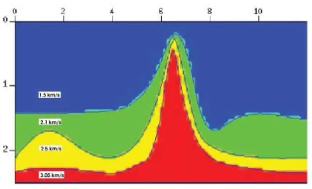
To test the refinements methods in extreme conditions, we gen-erated a model with strong geometrical changes. Figure (1) depicts a four layered acoustic model with three curved interfaces. Observe the geometrical variations near the middle of the model where the dips are
5 INTERSIS is a graphical interface for seismic modelling developed at the Laboratory of Computational Geophysics of the UNICAMP. The current version of INTERSIS allows to work with ray tracing and finite differences.
up to 67°. Simulated multicoverage acquisition was carried out over the entire profile using 200 shot records of 60 receivers each.
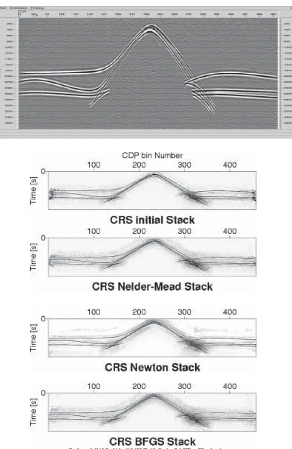
Regarding the stacked sections, Figure 2 shows the NMO stack, the CRS initial and the CRS Nelder-Mead, Newton and BFGS refined stacks. As a result of the strong dips in the model, the stacked sections
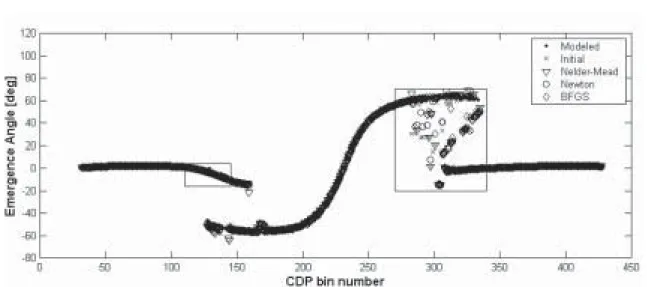
present a zone with caustics near CMP 300. As can be observed, there are not too many differences between these stacks. Figure 3 displays the modelled, initial and optimized emergence angle for the third reflector. The parameter curves for KNand KNIP have the same behavior as the one for β. As a consequence, we refrain from presenting them here.
Figure 1 – 2D isovelocity layered model. Horizontal distance and depth are in kilometers.
Figura 1 – Modelo com camadas de velocidade constante. Distâncias dadas em qiilometros e velocidades em km/s.
Table 1 – Q for the CRS parameters for each reflectors for Example 1. Tabela 1 – Q para os parâmetros CRS nos reflectores do modelo da Figura 1.
β
In Figure 4, we focus on the two boxes depicted in Figure 3. From the picture on the left, we observe that the optimization process may not improve the initial value of the parameter. The picture on the
right shows the angle values in the caustic region between CDPs 280-360. Table 1 summarizes the values of Q for the CRS parameters for each reflector.
Figure 2 – Synthetic stacks. The one in the top was obtained using ProMAX. Figura 2 – Seções empilhadas. A seção da superior foi obtida
Synthetic Example 2
This model has the objective of testing the refinement step for a more realistic case. Figure 5 depicts a four layer acoustic model with three curved interfaces. The acquisition parameters are the same as in the previous experiment.
As expected, the stacks obtained using the CMP and the CRS techniques are quite similar. For that reason, Figure 6 only shows the one obtained with CRS using Newton’s method at the refinement step. The differences between the parameter curves are not visible. The values for Q are indicated in Table 2.
Figure 3 – Modelled, initial and optimized emergence angles for the third reflector in Figure 1. The boxes are zoomed in Figure 4. Figura 3 – Ângulo de incidência do raio central (modelado, inicial e otimizado) para o terceiro refletor da Figura 1.
As caixas são ampliadas na Figura 4.
Figure 4 – Zoomed boxes (caustic regions) of Figure 3. Left box (km 2.7 to km 3.7 in the velocity model). Right box (km 7.0 to km 8.5 in the velocity model). Note that initial values may be closer to modelled ones than optimized values.
Figura 4 – Ampliações das caixas da figura anterior. Observe que os valores otimizados estão mais perto dos valores modelados que os iniciais.
From these two synthetic experiments, we observed that no mat-ter which method we use for the refinement step, the process has a smoothing effect over the CRS parameters. To illustrate this fact, Figure 7 depicts the initial and refined estimates of the emergence angle for the first reflector of the synthetic Example 2.
As a consequence of the smoothing effect, the stacks obtained with the refined parameters are, locally, smoother than the ones ob-tained with the initial parameters. This fact will be better observed in the next experiment with real data.
Figure 5 – 2D isovelocity layered model. Horizontal distance and depth are in kilometers. Velocities are in m/s. Figura 5 – Modelo com camadas de velocidades constantes. Distâncias dadas em quilometros e velocidades em km/s.
Figure 6 – Newton version of CRS stack of synthetic Example 2. Figura 6 – Seção empilhada e otimizada com o método de
Newton do modelo sintético da Figura 5.
Real Data
We have applied the refinement approach to a real marine dataset. Figure 8 shows the NMO stack, obtained from the commercial seismic software ProMAX, and the CRS stack using Newton’s method in the refinement step. The CRS stacks using the three refinements (Nelder-Mead, Newton and BFGS) are quite similar, and for that matter not
shown here. In fact, the BFGS provided a slightly smoother section, but not significant to justify a discussion here.
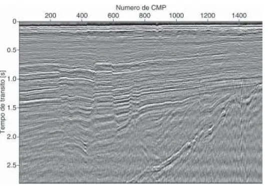
In the central part of the stacked sections, the CRS stack presents less aleatory noise, better continuity of the primaries and less quantity of reverberations. Due to these characteristics, the CRS stack is able to bet-ter define the unconformity that occurs between 1.3 s and 1.5 s all along the section.
Between CMPs 700 and 1500, the CRS stack has made more evident a probable basement structure. It is out of the scope of the present paper, however, to undertake a detailed investigation on the NMO and CRS stack results. Our aim here is just to point out that there are signifi-cant differences that require a better understanding and interpretation. As already mentioned, the initial step of the MULTISIS software adopts the same strategy as in Mann (2002). This strategy allows qua-lity control at the first search, that one applied on each CMP section of the dataset, called AUTOCMPSTACK. As this one-parameter search is equivalent to a conventional NMO stack, but with automatic picking of events that presents the higher coherences, the stack produced in this step is expected to look like the NMO stack. Regarding this stack, between CMPs 1300 and 1400 for t ≈ 1.5s, we find a horizontal event of
Figure 7 – Emergence angle for the first reflector of synthetic Example 2. The continuous line represent the refined values and the dots the initial estimative. Figura 7 – Ângulo de incidência do raio central para o primeiro refletor da Figura 5.
A linha contínua representa os valores otimizados, os pontos são os valores iniciais. Table 2 – Q for CRS parameters at reflectors for Example 2. Tabela 2 – Q para os parâmetros CRS nos reflectores do modelo da Figura 5.
β
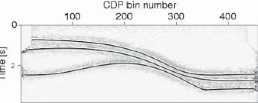
interest, as shown in the top of Figure 9. Taking a closer look to a CMP section in this range by means of a semblance map, we see that the AUTOCMPSTACK is stacking a back scattering energy, as indicated in Figure 10. This problem can be solved constraining the range for the search of the NMO velocity, and running again the AUTOCMPSTACK. The result is that the horizontal event disapears, as shown in the bottom of Figure 9.
Finally, regarding the smoothing effect commented in the syn-thetic experiments, we show in Figure 11 the stack obtained with the initial estimates of the CRS parameter and the one obtained after the refinement step using Newton’s method. The smoothing effect is clearly visible, confirming the observations made with the synthetic data.
Figure 8 – Marine real data stacks. Top: NMO (ProMAX). Bottom: CRS (Newton).
Figura 8 – Seções empilhadas de dados marinhos. Na parte superior a versão obtida com o pacote ProMAX, na parte inferior a versão CRS otimizada com o método de Newton.
Figure 9 – First and Corrected versions of the initial stack for the CRS stacking in Figure 8.
Figura 9 – Seções empilhadas inicial e corrigida da seção empilhada da Figura 8.
Figure 10 – Velocity analysis of CMP 1320. The higher semblance value near 1.5s (A) is most probably due to back scattering energy. The right value of velocity, (B), is about 2520m/s.
Figura 10 – Análise de velocidades para o CMP 1320. O valor alto da semblance perto dos 1.5s (A) é devido a reflexões laterais. O valor correto da velocidade (B) é 2520m/s.
Figure 11 – Effect of parameter refinement on real data stacks. Top: stack obtained with the initial estimative of the CRS parameter triplet. Bottom: stack obtained with a Newton refined CRS parameter triplet.
Figura 11 – Efeito do refinamento dos parâmetros no resultado final nas seções empilhadas. Na parte superior, seção inicial, na parte inferior, seção obtida com os parâmetros CRS otimizados usando o método de Newton.
CONCLUSIONS
We have provided an overview of the Common-Reflection-Sur-face (CRS) method, encompassing a brief description of both its theo-retical and implementation aspects. Our description considered the 2D situation in which sources and receivers were located on a single seismic horizontal line and the multicoverage data is aimed in producing, by stacking, a simulated ZO section. The CRS method uses a three-parameter hyperbolic traveltime moveout and the heart of the method is the esti-mation of these parameters.
The general strategy is to split the estimation into two steps. In the first step (initial), a quick estimation is performed using a suite of simplified versions of the problem. The next step (refinement) optimizes the parameters using the initial estimates and the full multicoverage data. Assuming that initial estimates of the parameters were given, we have examined three local optimization schemes to refine them, namely the Nelder-Mead, Newton and BFGS methods.
Our experiments show that the three refinement methods lead to similar stacked sections. The CRS, as well documented in the literature, produces, in general, sharper sections with less noise, as compared to the usually smoother NMO sections. Being a more automatic procedure, the CRS sections may, however, also enhance undesirable events such as multiples.
Regarding the estimation of the CRS parameters, our experiments show that, surprisingly, the refinement step may not always lead to better parameter estimates. Sometimes the refinement step may even lead to less accurate estimates. One possible reason for this behaviour is that the goal of the refinement step is to fit the best parameters to the hyperbolic moveout formula. However, the true values for the param-eters came from a Taylor’s interpolation. Therefore, depending on the aperture for the stacking, the fitted parameters can be quite different from the exact values. The same phenomena appears in the estimation of the NMO velocity from CMP gathers, as well explained in Castle (1994). At the moment we are engaged in more experiments and research to gain a better understanding on this subject.
Our tests with a real dataset showed a few significant differences between the CRS and NMO stacks. These differences, briefly addressed in the text, indicate the potential of the CRS method to be used in prac-tice. In fact, we hope that this work stimulates further investigations on
the CRS method, especially on the interpretative aspects of the obtained sections.
Acknowledgements
This work has been partially supported by the em National Council of Scientific and Technological Development (CNPq), Brazil, the Research Foundation of the State of São Paulo (FAPESP), Brazil, and the sponsors of the Wave Inversion Technology (WIT) Consortium. We also acknowl-edge the National Petroleum Agency (ANP), Brazil, for permission to show the marine real dataset used in this work. We finally thank E. Filpo and C. Guerra from PETROBRAS, Brazil, for helpful discussions and sug-gestions.
REFERENCES
BIRGIN, E. et al. Restricted optimization as a clue to fast and accurate implementation of the common reflection surface stack method. Journal of Applied Geophysics, [S.l.], v. 42, p. 143-155, 1999.
CASTLE, R. J. A theory of normal move out. Geophysics, [S.l.], v. 59, p. 983-999, 1994.
CHIRA-OLIVA, P. et al. Formula for a 2D curved measurement surface and finite-offset reflections. Journal of Seismic Exploration, [S.l.], v. 10, p. 245-262, 2001.
GARABITO, G. Empilhamento de superfícies de reflexão comum: uma nova seqüência de processamento usando otimização global e local. 2001. Tese (Doutorado)-Universidade Federal do Pará, Belém, 2001. GILL, P. E.; MURRAY, W.; WRIGHT, M. H. Pratical optimization. [S.l.]: Academic Press, 1981.
HUBRAL, P. Computing true amplitude reflections in a laterally inhomo-geneous earth. Geophysics, [S.l.], v. 48, p. 1051-1062, 1983. MANN, J. Extensions and application of the common reflection surface stack method. 2002. Thesis (PhD)-University of Karlsruhe, [S.l.], 2002. MÜLLER, J. The common reflection surface stack method: seismic imaging without explicit knowledge of the velocity model. 1999. Thesis (PhD)-University of Karlsruhe, [S.l.], 1999.
NEIDEL, N.; TANER, M. Semblance and other coherency measures for multichannel data. Geophysics, [S.l.], v. 36, p. 482-497, 1971.