Rev Saúde Pública 2009;43(1)
Mery Natali Silva AbreuI,II Arminda Lucia SiqueiraIII Waleska Teixeira CaiaffaI,II
I Programa de Pós-graduação em Saúde
Pública. Faculdade de Medicina (FM). Universidade Federal de Minas Gerais (UFMG). Belo Horizonte, MG, Brasil
II Grupo de Pesquisa em Epidemiologia e
Observatório de Saúde Urbana. FM-UFMG. Belo Horizonte, MG, Brasil
III Departamento de Estatística. Instituto de
Ciências Exatas. UFMG. Belo Horizonte, MG, Brasil
Correspondence: Mery Natali Silva Abreu Av. Alfredo Balena, 190, 6º andar Sala 625 Santa Efi gênia
31130-100 Belo Horizonte, MG, Brasil E-mail: [email protected] Received: 5/10/2007
Revised: 5/23/2008 Approved: 6/11/2008
Ordinal logistic regression in
epidemiological studies
ABSTRACT
Ordinal logistic regression models have been developed for analysis of epidemiological studies. However, the adequacy of such models for adjustment has so far received little attention. In this article, we reviewed the most important ordinal regression models and common approaches used to verify goodness-of-fi t, using R or Stata programs. We performed formal and graphical analyses to compare ordinal models using data sets on health conditions from the National Health and Nutrition Examination Survey (NHANES II).
DESCRIPTORS: Statistics as Topic. Logistic Models. Regression Analysis. Epidemiologic Methods.
INTRODUCTION
Ordinal logistic regression models have been applied over the last few years for analyzing data, the response or outcome of which is presented in ordered categories. Ordered information in score-form has been increasingly used in epidemiological studies, such as quality of life in interval scales, health condition indicators and even for indicating the seriousness of illnesses.1 Depending on
the study’s purpose, these models also allow the odds ratio (OR) statistic or the probability of the occurrence of an event to be calculated.1
There are several ordinal models, such as the proportional odds, partial pro-portional odds, continuation-ratio and stereotype logistic models. Despite this diversity and the great variety of studies1-4,7-15 on the subject their use in the
public health area is still rare.1 This may be attributed not only to their
comple-xity, but specially to the diffi culty encountered when it comes to validating their assumptions.11 Another factor that may be related to the limited use of these
models is the reduced number of modeling options offered in the commercial statistical packages used in the public health area, examples being SPSS and Minitab. Even if other, more complex packages are used, such as SAS and Stata, it is frequently diffi cult to select the appropriate commands and to interpret the results.3 Added to these diffi culties is the considerable cost of the majority of
the commercial statistical packages available, because access to their licenses is highly restricted.
One statistical package that has become more and more popular is the free software R,6,a which is distributed under a general public license. The
pa-ckage contains a variety of statistical techniques, including several ordinal logistic regression models, which allow them to be tested and adjustments to be compared.
Comments
a The R Project for Statistical Computing [internet]. Viena: Viena University of Economics and Business
The aim was this article was to analyze the adjustment and adaptation of the main ordinal regression models and show the commands used in the R software. In addi-tion to this assessment/analysis the partial proporaddi-tional odds model was adjusted, using Stata software, because it has not yet been included in the R software.
To provide examples for the methods analyzed, some of the data from the well-known Second National Health and Nutrition Examination Survey (NHANES II) will be used. This survey is available on the internetb and
it is widely used as examples in statistical and epide-miological studies. The survey includes demographic, anthropometric, nutritional history, health and hema-tology information. Information in the database about children, extracted from 10,337 interviews with people between the ages of 20 and 74, was excluded.
UNIVARIATE ANALYSIS
As in any analytical procedure that uses regression models, multiple analysis using ordinal models must always be preceded by comparing each covariable with the event of interest being investigated. By means of this analysis, which is known as univariate, it is possi-ble to select the factors that will be introduced into the regression model.
The chi-squared test for trend is one of those that is suitable for selecting principal effects, since it considers the ordinal nature of the response variable. Normally, a conservative level of signifi cance is used (generally between 10% and 25%) for entering the covariables in the model.10
Furthermore, OR can be estimated considering one res-ponse variable category as a reference point and compa-ring it with the others or grouping the larger categories and comparing them with the smaller categories.
ORDINAL REGRESSION MODELS
After univariate analysis, the fi nal multiple regression model should be constructed to control possible con-fusion factors. As the event of interest is ordinal, an ordinal logistic regression model must be used.
Let Y be the response variable with k categories codifi ed
as 1,2,...,k and the vector of the
explanatory variables or covariables. The k categories of Y that are conditional on the values occur with probabilities p1, p2,... , pk, in other words pj = P(Y =j), for j=1, 2,...k. The term α refers to the intercept of the model and corresponds to the effects of the covaria-bles on the response variable. Table 1 gives the forms
a National Center for Health Statistics. Publications and Information Products: NHANES II public-use and data fi les. [cited 2008 Nov 11]
Available from: http://www.cdc.gov/nchs/products/elec_prods/subject/nhanesii.htm
of the main models, an indication of their use and their commands in the R and Stata packages.
Proportional odds model (POM)
In the MOP (k - 1) cut-off points of the categories are considered, with the jth (j=1,..., k-1) cut-off point being based on a comparison of the accumulated probabilities, as shown in Table 1.
The term αj varies for each of the k categories and each does not depend on the j index, implying that the rela-tion between and Y is independent of the category.
Therefore, the model has a proportional odds assump-tion around the (k-1) cut-off points, also called the parallel regression assumption, which is assumed for each covariable included in the model. This assumption must be tested for each covariable separately and in the
fi nal model, using for example the score test.10
This model is suitable for analyzing ordinal variables arising from a continuous variable, which in turn has been grouped.
Partial proportional odds model (PPOM)
As the proportional odds assumption is diffi cult to achieve in practice, the PPOM may be used as an al-ternative.13 This model allows some covariables with
the proportional odds assumption to be modeled, but for those variables in which this assumption is not satisfi ed it is increased by a coeffi cient ( ), which is the effect associated with each jth cumulative logit, adjusted by the other covariables.10 The general form
of the model is the same as the previous one, but now the coeffi cients are associated with each category of the response variable.
It is normally expected that there will be a type of linear trend between each OR of the specifi c cut-off points and the response variable.1 If there is then a set
of restrictions ( kl) may be included in the model to clarify this linearity (Table 1). When these restrictions are included this model is called the restricted partial proportional odds model.
The τj parameters are fi xed scale parameters which take the form of restrictions allocated to the parameters. In this case for a given covariable Xm, αm does not depend on the cut-off points, but is multiplied by τj for each jth logit.11
Continuous ratio model (CRM)
3
Rev Saúde Pública 2009;43(1)
Table 1. Information about ordinal logistic regression models, indication of use, and commands when applying the R and Stata, using NHANES II as an example.
Model Functional form of the model Use indication R commands* Stata
commands
POM
Variable response, originally continuous and then grouped and proportional chances assumption is valid
> library (Design)
>mcp=lrm (health-age + diabetes + color_ skin,nhanes,x,TRUE,y=TRUE)
>mcp > par(mfrow=c(1,5))
> residuals (mcp, type = ‘score.binary’, pl=TRUE) > residuals (mcp, type= ‘partial’, pl=TRUE)
.ologit Health age
diabetes color_
skin
PPOM-NR When proportional chances
assumption is not valid
-.gologit2 Health age color_skin diabetes Autofi t lrforce PPOM-R
Proportional chances assumption is not valid and
there is a linear relation between OR of a covariable
and the response variable
CRM
There is an intrinsic interest in a specifi c category of the
response variable
>cr=cr.setup (nhanes$health) Health.cr=cr$cohort
Cohort=cr$cohort Age.cr=agelcr$subs Diabetes.cr=diabetes[cr$subs]
Color.cr=color_skin[cr$subs] Crm=lrm(health.cr+diabetes.cr+color,cr+cohort)
>crm
.ocratio Health age
diabetes color_skin
SE
Discrete ordinal response variable that does not come from any grouped
continuous variable
>install.packages
(“VGAM”,response=”http//www.stat.auckland. Ac.nz/-yee”)
>library/(VGAM)
Ms=mvglm(health~age+diabetes+color_skin, Nhanes,multinomial)
>summary/(ms)
.slogit Health age
diabetes color_skin
POM= Proportional odds model; PPOM-NR = Non-restricted proportional odds model; PPOM-R= Restricted proportional odds model; CRM=Continuous ratio model; SE = Stereotype model *NHANES study – variable response: health; covariables: age, diabetes and color_skin
a certain score, let us say yj, Y = j, with the probability of a greater response, Y > yj, as indicated in Table 1.
This model has different intercepts and coeffi cients for each comparison and can be adjusted for k binary logistic regression models.11 It is more suitable when
there is an intrinsic interest in a specifi c category of the response variable.1
Stereotype model (SM)
The SM can be considered an extension of the multi-nomial regression model.10 It compares each category
of the response variable with a reference category, normally the fi rst or last category. But, due to the ordinal nature of the data a linear structure is imposed on jl
(j=1,...,k e l=1,...,p), in other words, weights (ωj) are
attributed to the coeffi cients.11
The weights (ωj) of the model are directly related to the effect of the covariables. Because of this the OR will tend to grow, since the weights are normally constructed in an ordered manner
(0 = ω1 ≤ω2 ≤... ωk)
This model should be used when the response variable is an ordinal variable with discrete categories.
In all the ordinal models mentioned the signifi cance of the coeffi cients should be tested using the Wald test.10 In
the exercise presented it was calculated using approxi-mation by the normal standardized distribution.
CHECKING THE QUALITY OF THE ADJUSTMENT OF THE ORDINAL MODELS
As in any type of regression analysis, it is important to assess the quality of the adjustment of the ordinal logistic regression models, because failure to adjust may, for example, lead to a bias in the estimation of the effects. Assessment of the adjustment may detect: important covariables; interactions that were omitted; cases in which the linking function (logit) was not appropriated; cases in which the functional form of the modeling of the covariables is not correct; and
fi nally, cases in which there has been a violation of the proportional odds assumption.4
Although many methods have been developed for evaluating the adjustment of binary logistic regression models, few of these methods have been extended to ordinal response data.10 Normally, the quality of the
ad-justment of ordinal models is checked using the Pearson or deviance tests. These tests involve the constitution of a contingency table in which the lines comprise all the possible confi gurations of the covariables of the model and the columns are the categories of the ordinal response.14
The expected counts of this table are expressed as
, where Nl is the total number of individu-als classifi ed in line l and represents the probability of an individual in line l having the response j calcu-lated from the model adopted.14 The Pearson test for
evaluating the suitability of the adjustment compares these expected counts with those actually observed, using the formula:
(1)
The deviance statistic also compares observed and expected counts, but using the formula:
(2)
Tests used for evaluating the quality of the adjustment of the model are based on an approximation of the statistics (1) and (2) for the chi-squared distribution with (L-1)(k-1)p degrees of freedom (L is the number of lines, k is the number of columns in the contingency table and p is the number of covariables in the model). A signifi cant p-value leads to the conclusion of a lack of adjustment of the model to the data being studied.14
Pulkstenis & Robinson14 (2004) report that statistics
(1) and (2) do not provide a good approximation of the chi-squared distribution when continuous covariables are adjusted. They suggest small modifi cations in this case.
In this study, in all the models considered, Pearson or deviance adjustment quality tests were used, since they are found in the usual statistical packages.
As the literature on adjustment diagnosis or evaluation tools for ordinal models is relatively scarce, Hosmer & Lemeshow10 (2000) suggest the use of binary
regres-sions, separated for each cut-off point, thus creating diagnosis statistics for the ordinal models. Residual graphs are normally constructed for proportional odds models using the adjustment of these models to predict a series of binary events Y>j, j=1,2,...,k. Therefore, for the indicator variable [Y e” j], the residual score for case i and covariable p is given by:9
(3)
5
Rev Saúde Pública 2009;43(1)
each category of the response variable should have a similar appearance.9
Partial residuals are also widely used for checking if all the covariables of the model have linear behavior. In the context of ordinal regression, it is necessary to calculate binary logistic regression models for all the cut-off points of the response variable Y, with the par-tial residual for each case i and the covariable p being defi ned in the following way:9
(4)
The partial residual graphs provide estimates of how each covariable (x) relates to each category of response variable (Y).9
So partial residuals are used to check the need for changes in the covariables (linearity) or even the
vali-dity of the proportional odds assumption (parallelism of the curves).9
COMMANDS USED IN THE MODELS
In this section, the steps for adjusting the models in Section 2 in the R or Stata software that was summa-rized in Table 1 will be shown.
The commands were illustrated with data taken from NHANES II and the variables were called:
Response variable: health
Covariables: age, diabetes, skin color
Adjustment of the Models in R software
A) Proportional odds model
In the R software, the POM can be adjusted using the command lrm, developed by Harrell and forming part of the Design package (Table 1). This command adjusts
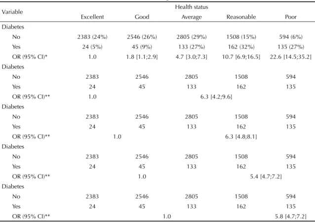
Table 2. Association between diabetes and health status, according to OR estimates and 95% confi dence intervals.
Variable Health status
Excellent Good Average Reasonable Poor Diabetes
No 2383 (24%) 2546 (26%) 2805 (29%) 1508 (15%) 594 (6%)
Yes 24 (5%) 45 (9%) 133 (27%) 162 (32%) 135 (27%) OR (95% CI)* 1.0 1.8 [1.1;2.9] 4.7 [3.0;7.3] 10.7 [6.9;16.5] 22.6 [14.5;35.2] Diabetes
No 2383 2546 2805 1508 594
Yes 24 45 133 162 135
OR (95% CI)** 1.0 6.3 [4.2;9.6]
Diabetes
No 2383 2546 2805 1508 594
Yes 24 45 133 162 135
OR (95% CI)** 1.0 6.3 [4.8;8.1]
Diabetes
No 2383 2546 2805 1508 594
Yes 24 45 133 162 135
OR (95% CI)** 1.0 5.4 [4.7;7.2]
Diabetes
No 2383 2546 2805 1508 594
Yes 24 45 133 162 135
OR (95% CI)** 1.0 5.8 [4.7;7.2]
* OR considering one category as a reference point (where Y = state of health; YD = excellent category, x(a) = no diabetes.
X(b) = suffering from diabetes
binary and ordinal proportional odds models using the maximum verisimilitude method or alternatively the penalized maximum verisimilitude method.9
The arguments used are: formula, in other words the terms to be included in the model (variable response and covariables) and fi le name, for the data to be used, etc. The outcomes shown after using the commands are: expression used, the frequency table for the res-ponse, vector with some important statistics, estimates of the coeffi cients, vector of the fi rst estimates derived from the verisimilitude function log and the deviance of the model.
B) Continuous ratio model
The CRM may be implemented in R software by res-tructuring the data, which is done using the cr.setup
command, which forms part of the Design package. This command makes it possible to create new varia-bles from the response variable y, which will be used to adjust the continuous ratio model.1
Four new variables are added with this command:
y – new binary variable that will be used as a response in adjusting the binary logistic regression model;
cohort – a vector indicating which cut-off point (two comparisons of the CRM) was applied;
subs – a vector used to replicate the other variables (explanatory) in the same way that y was replicated;
reps – a variable that specifi es how many times each original observation was replicated.
The model is obtained by adjusting a binary logistic regression in the restructured data with a new dichoto-mous response (y) as a dependent variable, including the created covariable (cohort), which indicates the le-vel of the cut-off point, and restructuring the covariables by the vector (subs), as shown in Table 1.1
The assumption of the heterogeneity of the cut-off points can be tested by including an interaction term in the model between the interest declaration and the indicator variable of the cut-off point (cohort). This is called the saturated model. The log value of the verisi-militude function of the models can be compared both with and without the interaction term.
C) Stereotype model
The SM can be adjusted using generalized linear models that have estimated restriction matrixes. The weights (restrictions) are estimated as additional parameters of the model, using the multinomial family for the adjustment.
In the R software, the SM can be adjusted using the command rrvglm that forms part of the VGAM package.17
Residual analysis
The Design package function residuals.lrm is used to construct residual graphs after adjusting the POM in the R software, as shown in Table 1.
In the score residual graph (score.binary), if the pro-portional odds assumption is valid, it is expected that for each covariable, the trend of the response variable categories will be constant on the horizontal line. In the partial residual graph (partial), on the other hand, in a well-adjusted model it is expected that the curves will be both linear and parallel.9
Stata software
Adjustment of the partial proportional odds model
So far the PPOM is not available in R software, but it can be adjusted in Stata 9.0 using the command gologit2
developed by Williams16 (2006). This command made
Table 3. Results* of the fi nal proportional odds model**, according to the health status response (NHANES II)
Covariable β EP(β) OR P-value score test***
Diabetes
0.60
No 1.00
Yes 1.26 0.09 3.35
Skin color
0.01
Non-white 1.00
White -0.86 0.14 0.42
Other -0.64 0.06 0.53
Age (in years) 0.04 0.01 1.04 <0.01
* In all models all the variables were signifi cant at the 1% level ** Final p-value score test (value-p<0.001)
7
Rev Saúde Pública 2009;43(1)
it possible to test the proportional odds assumption, using the autofi t option and adjusting coeffi cients for the various variable categories in which this assumption is violated.
APPLICATION EXAMPLE - NHANES II
As a dependent variable, state of health classifi ed into
fi ve categories was considered: (1= poor, 2=reasonable, 3=average, 4=good and 5=excellent). Didactically, a model was constructed using three explanatory variables: a quantitative variable – age (in years), a categorical binary variable – diabetes (no; yes) and a variable with more than two categories – skin color (white; non-white; other). For the skin color variable indicator variables were created, considering non-white as a point of reference.
Table 2 was constructed as a didactic way of showing how OR can be obtained, considering a category as the reference or grouping the categories. In the fi rst calcu-lation “excellent” state of health was considered as the reference point and each of the subsequent categories was compared with it separately, as was done in the SM. The value of OR is seen to increase as the state of health deteriorates.
In the second calculation, OR was calculated in accor-dance with the POM equation, in which smaller or equal values are compared with a given category with larger values (Table 1). When compared with the “excellent” state of health, the OR of the states “good” and “poor” (OR=6.3) was equal to when we compared “excellent” and “good” states of health with “average”, “reasona-ble” and “poor” states. This case is an example of the proportional odds model, in other words, with an OR similar for all categories compared, which is the main assumption of the POM.
The POM results are shown in Table 3. The test score suggests there is violation of the proportional odds assumption for the variables “skin color” and “age”, in isolation, and also for the multiple model. Fur-thermore, the deviance test indicated that the model lacked adjustment.
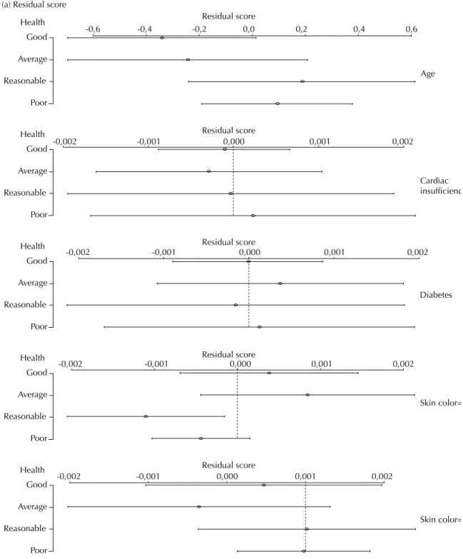
The residual graphs (score and partial) for evaluating the suitability of the POM are shown in Figures 1 and 2, respectively. In Figure 1 (residual score), the results reinforce the conclusion of the score test, because the curves for the “diabetes” variable showed a horizontal format close to zero. However, the “age” variable beha-vior oscillated for the “good” and “average” states of health categories and is well below the line of the zero residual. The same happened with the covariable “skin color”. But in this case, the biggest oscillation was seen in the “reasonable” and “poor” states of health catego-ries for the classifi cation “others” and in the “average” category for the color “white”.
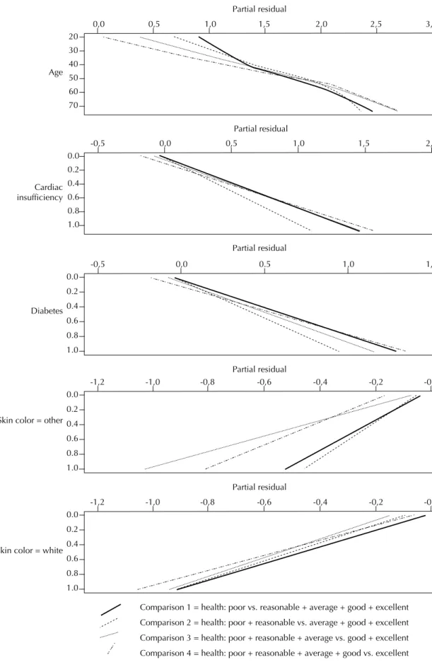
In the partial residual graphs (Figure 2), the assump-tion of parallel regression seemed very acceptable due to its linear aspect and because of the approximately parallel straight lines for the variable “diabetes”. In the “others” category graph of the variable “skin color”, on the other hand, despite its linear behavior, the curves crossed, therefore violating the assumption of paralle-lism. There was no linear behavior with the covariable “age”, which might contribute to the lack of adjustment of the model. Even when higher degree terms for “age” were included, the deviance test continued to indicate poor adjustment.
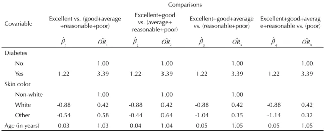
Adjustment of the PPOM is shown in Table 4. In this model, the effects were signifi cant for the four compa-risons and the coeffi cients did not vary for the variable “diabetes”, indicating that an individual with a worse state of health has 3.39 times more chance of being diabetic, when compared with an individual whose state of health is better.
Compared to the “non-white” skin color, there was no variation in the coeffi cients in the various comparisons for skin color “white”, while for “other” skin color there was a variation. As worse states of health were evaluated, there was an increase in the protection effect, i.e., there was a reduction in the absolute value of OR. For the covariable “age”, a change in the size of OR was also seen in various categories when comparing states of health. For every additional year in age, the chance of the state of health moving from good to poor was 1.03 times higher that with a person in an excel-lent state of health. This chance can reach 1.05 times when someone with a poor state of health is compared with someone with excellent health moving to having reasonable health.
As for SM, in all comparisons, the effect of the co-variables was significant (value-p<0,01), and the deviance test indicated there was good adjustment of the model (Table 5). In other words, people with poor health have ten times more chance of being diabetic than those who are in excellent health. The magnitude of this association reduces as the state of health gets close to excellent, reaching 1.43 in the comparison of good health with excellent health.
COMMENTS
Generally speaking, ordinal logistic regression models are recommended for analyzing ordinal data.1,3,8,10,11
Ananth & Kleinbaum1 (1997) report that the POM and
CRM are the most widely used in epidemiological and biomedical applications in relation to PPOM and SM. But these models lead to strong assumptions that, if they are not valid, may lead to incorrect interpretations, as occurred in the example used.1
Other authors11 state that the type of model used
de-pends on the character of the ordinal response variable, i.e., whether this variable was ordered starting with a regrouped continuous variable or if it originated from a discrete variable. In the fi rst case, the POM is the most indicated when the premise of parallel straight lines is not violated. In the second case, the SM is the most indicated, as in this study, in which the response
Age
Health Residual score
-0,6 -0,4 -0,2 0,0 0,2 0,4 0,6
Good
Average
Reasonable
Poor
-0,002 -0,001 0,000 0,001 0,002
Residual score
Cardiac insufficienc
-0,002 -0,001 0,000 0,001 0,002
Residual score
Diabetes
-0,002 -0,001 0,000 0,001 0,002
Residual score
Skin color=
-0,002 -0,001 0,000 0,001 0,002
Residual score
Skin color= Health
Good
Average
Reasonable
Poor
Health
Good
Average
Reasonable
Poor
Health Good
Average
Reasonable
Poor
Health Good
Average
Reasonable
Poor
9
Rev Saúde Pública 2009;43(1)
Figure 2. Residual graphs (score and partial) for the covariables included in the model, according to the health status response. Comparison 1 = health: poor vs. reasonable + average + good + excellent
Comparison 2 = health: poor + reasonable vs. average + good + excellent
Comparison 3 = health: poor + reasonable + average vs. good + excellent
Comparison 4 = health: poor + reasonable + average + good vs. excellent Partial residual
-1,0 -0,6
0.0
0.2
0.4
0.6
0.8 1.0
-0,8
-1,2 -0,4 -0,2 -0,
Skin color = white
Partial residual
-1,0 -0,6
0.0
0.2
0.4
0.6 0.8
1.0
-0,8
-1,2 -0,4 -0,2 -0,
Skin color = other
Partial residual
0,0 0.5 1,0 1,5
0.0
0.2
0.4
0.6 0.8
1.0 -0,5
Diabetes
Partial residual
0,0 0,5 1,0 1,5 2,0 2,5 3,0
20 30 40 50 60 70 Age
0,0 0,5 1,0 1,5 2,0
0.0 0.2 0.4 0.6 0.8 1.0
-0,5
Cardiac insufficiency
variable, defi ned as state of health in the NHANES II study was treated with discrete categories.
Even in the presence of an ordinal response, other multivariate analysis options should be considered. One way is to use the decision-tree method,5 which is a more
descriptive method that considers a greater number of variables in the fi nal model. Other linking functions of the model may also be used, like probit analyses and complementary log-log. However, ordinal regression is a parametric technique that, by imposing a rigid, more conservative and economical structure on the model, allows the reliability intervals for the parameters to be quantifi ed; this makes it easier to interpret the OR. While alternative approaches are worth analyzing and discussing, they will not be discussed in this article.
In constructing ordinal models, Hosmer & Lemeshow10
(2000) propose strategies like those used in the example
in this article. These authors initially recommend car-rying out a univariate analysis for selecting the principal effects and including in the model just signifi cant varia-bles that have a prefi xed level of signifi cance. Then, the model should be adjusted, its suitability checked using appropriate tests and residual graphs and fi nally the model should be interpreted by estimating the OR.
However, there are few methods for checking the ad-justment of ordinal models. In the literature available we have so far found no technique for checking the adjustments of the SM. The existing diagnosis statistics proposed by Harrel9 (2002) and applicable to the POM,
are merely graphs taken from binary regressions, sepa-rated for the ordinal variable cut-off points. Although they are incomplete, these techniques are extremely important when it comes to getting an indication of the quality of the adjustment of ordinal models. Analysis of partial residuals, even when graphic, is considered Table 4. Results* of the fi nal partial proportional odds model, according to the health status response (NHANES II).
Covariable
Comparisons
Excellent vs. (good+average +reasonable+poor)
Excellent+good vs. (average+ reasonable+poor)
Excellent+good+average vs. (reasonable+poor)
Excellent+good+averag e+reasonable vs. (poor)
1 1 2 2 3 3 4 4
Diabetes
No 1.00 1.00 1.00 1.00
Yes 1.22 3.39 1.22 3.39 1.22 3.39 1.22 3.39
Skin color
Non-white 1.00 1.00 1.00
White -0.88 0.42 -0.88 0.42 -0.88 0.42 -0.88 0.42
Other -0.54 0.58 -0.44 0.64 -1.04 0.35 -1.14 0.32
Age (in years) 0.03 1.03 0.04 1.04 0.05 1.05 0.05 1.05 * In all models all the variables were signifi cant at the 1% level
Table 5. Results* of the fi nal stereotype model**, according to the health status response (NHANES II)
Covariable
Comparisons of state of health
Poor vs. excellent Reasonable vs.
excellent Average vs. excellent Good vs. excellent
1 1 2 2 3 3 4 4
Diabetes
No 1.00 1.00 1.00 1.00
Yes 2.25 9.45 1.69 5.43 0.97 2.64 0.36 1.43
Skin color
Non-white 1.00 1.00 1.00 1.00
White -1.64 0.19 -1.23 0.29 -0.71 0.49 -0.26 0.77
Other -1.30 0.27 -0.98 0.38 -0.56 0.57 -0.21 0.81
Age (years) 0.08 1.08 0.06 1.06 0.03 1.03 0.01 1.01 * In all models all the variables were signifi cant at 1% level.
11
Rev Saúde Pública 2009;43(1)
very useful for ordinal models, because they check both linearity, indicating possible changes that should be used, and the proportional odds assumption.
On the other hand, care must be taken when interpreting residuals, principally considering once again the lack of information of how to do it. Sometimes, the graphs may suggest confusing information and make it diffi cult to take decisions as to whether the proportional odds assumption has been violated or not. An alternative is to use residual analysis along with the score test, because when there is any doubt as to the format of the graph this test may contribute to a fi nal conclusion being reached.
Ordinal logistic regression models have shown to be suitable for analyzing data with ordinal response. The choice of the best model depends on the character of the ordinal variable, adaptation of the model to the assumptions, the quality of the adjustment and the capacity it has for coming up with a good explanation with a reduced number of parameters to be estimated.
Finally, when it comes to using ordinal models, good computer skills and mastery of the commands are essen-tial, not only for choosing the most suitable model but also for making comparisons between models. For this reason, the R program, which includes various models and some diagnosis graphs, is an important tool.9
1. Ananth CV, Kleinbaum DG. Regression models for ordinal responses: a review of methods and applications. Int J Epidemiol. 1997;26(6):1323-33. DOI: 10.1093/ije/26.6.1323
2. Anderson JA. Regression and ordered categorical variables. J R Statist Soc B. 1984,46(1):1-30.
3. Bender R, Benner A. Calculating ordinal regression models in SAS and S-Plus. Biometrical J. 2000;42(6):677-99. DOI: 10.1002/1521-4036(200010)42:6<677::AID-BIMJ677>3.0.CO;2-O
4. Brant R. Assessing proportionality in the proportional odds model for ordinal logistic regression. Biometrics. 1990;46(4):1171-8. DOI: 10.2307/2532457
5. Breiman L, Friedman J, Stone CJ, Olshen RA. Classifi cation and regression trees. New York: Chapman & Hall; 1984.
6. Colin RB. Bioestatística usando R: apostila para biólogos. Bragança; 2004.
7. Fienberg SE. Fixed Margins and Logit Models. In: Fienberg SE. The analysis of cross-classifi ed categorical data. Cambridge, MA: MIT Press; 1980. p.110-6.
8. Greenland S. Alternative models for ordinal logistic regression. Stat Med. 1994;13(16):1665-77. DOI: 10.1002/sim.4780131607
9. Harrell Jr FE. Regression modelling strategies: with applications to linear models, logistic regression, and survival analysis. New York: Springer; 2002.
10. Hosmer DW, Lemeshow S. Applied logistic regression. 2. ed. New York: John Wiley & Sons; 2000.
11. Lall R, Campbell MJ, Walters SJ, Morgan K. A review of ordinal regression models applied on health-related quality of life assessments. Stat Methods Med Res. 2002;11(1):49-67. DOI: 10.1191/0962280202sm 271ra
12. McCullagh P. Regression models for ordinal data. J R Statist Soc B. 1980;42(2):109-42.
13. Peterson BL, Hanrrel FE. Partial proportional odds models for ordinal response variables. Appl Statistic. 1990;39(2):205-17. DOI: 10.2307/2347760
14. Pulkstenis E, Robinson TJ. Goodness-of-fi t tests for ordinal response regression models. Stat Med. 2004;23(6):999-1014. DOI: 10.1002/sim.1659
15. Walker SH, Ducan DB. Estimation of the probability of an event as a function of several independent variables. Biometrika. 1967;549(1):167-79.
16. Williams R. Generalized ordered logit/partial proportional odds models for ordinal dependent variables. Stata J. 2006;6(1):58-82.
17. Yee TW, Hastie TJ. Reduced-rank vector generalized linear models. Statist Model. 2003;3(1):15-41. DOI: 10.1191/1471082X03st045oa
REFERENCES