OF ENVIRONMENTAL VARIABLES
Antonio Carlos Ferraz Filho1, José Roberto Soares Scolforo2, Maria Zélia Ferreira3, Romualdo Maestri4, Adriana Leandra de Assis5, Antônio Donizette de Oliveira6, José Márcio de Mello7
(received: June 26, 2009; accepted: May 27, 2011)
ABSTRACT: This study investigated the behavior of climatic variables inserted as inclination modifi ers of the Chapman-Richards model for estimating dominant height. Thus, 1507 data pairs from a Continuous Forestry Inventory of clonal eucalyptus stands were used. The stands are located in the States of Espírito Santo and southern Bahia. The climatic variables were inserted in the dominant height model because the model is a key variable in the whole prognosis system. The models were adjusted using 1360 data pairs, where the rest of the data was reserved for model validation. The climatic variables were selected by using the Backward model construction method. The climatic variables indicated by the Backward method and inserted in the model were: mean monthly precipitation and solar radiation. The inclusion of climatic variables in the model resulted in a precision gain of 19.8% for dominant height projection values when compared with the conventional model. The advantage of the method used in this study is the actualization of inventory data contemplating climatic history and productivity estimates in areas without prior plantation.
Key words: Climatic variable, dominant height, projection model.
MODELO DE PROJEÇÃO EM ALTURA DOMINANTE COM ADIÇÃO DE VARIÁVEIS AMBIENTAIS
RESUMO: Conduziu-se este estudo, com a fi nalidade de avaliar o efeito da introdução de variáveis ambientais introduzidas como modifi cadores da inclinação do modelo de Chapman-Richards, para a projeção de altura dominante. Para isso foram utilizados 1507 pares de dados de IFC provenientes de plantios clonais de eucalipto, localizados nos Estados do Espírito Santo e sul da Bahia. As variáveis ambientais foram introduzidas no modelo de altura dominante por ser essa variável chave em todo o sistema de prognose. O ajuste dos modelos foi realizado com 1360 pares de dados, sendo que o restante dos dados foram reservados para a validação do modelo. A escolha das variáveis ambientais foi feita pelo método de construção de modelos Backward. As variáveis ambientais indicadas pelo método Backward e inseridas no modelo de projeção foram: precipitação mensal média e radiação solar média. O ganho com a inclusão das variáveis climáticas na precisão das projeções da altura dominante foi de 19,8% em relação ao modelo sem variável ambiental. A metodologia de modelagem utilizada neste trabalho apresenta a vantagem de poder atualizar inventários com base no histórico climático e estimar produtividade em locais sem histórico de plantios.
Palavras-chave: Variável climática, altura dominante, modelo de projeção.
1Forest Engineer, Ph.D. candidate in Forest Science – Departamento de Ciências Florestais – Universidade Federal de Lavras – Cx. P. 3037 – 37200-000 –
Lavras, MG, Brasil – acferrazfi lho@gmail.com
2Forest Engineer, Professor Ph.D. in Forest Science – Departamento de Ciências Florestais – Universidade Federal de Lavras – Cx. P. 3037 – 37200-000 –
Lavras, MG, Brasil – scolforo@dcf.ufl a.br
3Forest Engineer, Ph.D. in Forest Science – Veracel Celulose S.A – Cx. P. 23 – 45820-970 – Eunápolis, BA, Brasil – maria.zelia@veracel.com.br
4Forest Engineer, Ph.D. in Forest Science – Grandfl or – R. João Manoel, 1448 – 97300-970 – São Gabriel, RS, Brasil – rm@grandfl or.com.br
5Forest Engineer, Ph.D. in Forest Science – Fibria S. A. – Rodovia Aracruz-Barra do Riacho, s/nº, Km 25 – 29197-000 – Aracruz, ES, Brasil –
alassis@fi bria.com.br
6Forest Engineer, Professor, Ph.D. in Forest Science – Departamento de Ciências Florestais – Universidade Federal de Lavras – Cx. P. 3037 – 37200-000 –
Lavras, MG, Brasil – donizete@dcf.ufl a.br
7Forest Engineer, Professor, Ph.D. in Forest Resources – Departamento de Ciências Florestais – Universidade Federal de Lavras – Cx. P. 3037 –
37200-000 – Lavras, MG, Brasil – josemarcio@dcf.ufl a.br
1 INTRODUCTION
With the development of the Brazilian forest sector and the market’s increase in demand for wood products, the application of adequate techniques of forest inventories and management is fundamental to realize a complete and precise diagnosis of forest yield. Thus, the use of such techniques will positively infl uence planning and
composition and structure. Common usage of the term “growth model” generally refers to a system of equations which can predict the growth and yield of a forest stand under a wide variety of conditions. Thus, a growth model may comprise a series of mathematical equations, the numerical values embedded in those equations, the logic necessary to link these equations in a meaningful way, and the computer code required to implement the model on a computer.
Models can be either mechanistic (process based) or empirical (SCOLFORO, 2006). Mechanistic models attempt to estimate forest growth using edafi c, physiological and environmental processes that directly affect growth. Therefore, they are more general models in the sense that they can be applied to estimate the potential productivity in areas without forest and under changing environmental conditions, in other words, they can be used to predict data beyond the observed range used to generate the model. The limitations to apply mechanistic models as a practical tool are due to a large number of parameter values and its complexity.
Due to their simplicity, empirical models are widely used as practical tool by forest managers. These models are calibrated on a forest’s permanent plot data (e.g. age, site expressed as height and basal area), capturing consequences and not causes of physiological processes, in this case forest growth. As a result, they are very precise when predicting data in the observed range used to calibrate the model, but tend to be biased when used as a prediction tool outside the observed range.
A hybrid approach combining the main advantages of the process based and empirical models model is being adopted in some circumstances. Snowdon et al. (1998) used climatic indices derived from a mechanistic model, BIOMASS, into an empirical growth model to describe stand height, basal area and volume in a spacing trial with
Pinus radiata, improving the fi t compared to the basic
equation by 13%, 22% and 31% for mean tree height, stand basal area and stand volume, respectively. Almeida et al. (2002) demonstrated the possibility of integrating the process-based model 3-PG, which estimates forest growth using climatic data and stand characteristics, with the empirical model E-GROW ARCEL, which estimates forest growth recovering parameters of the Weibull probability density function and therefore providing estimates by diameter class. The link between these two models was realized by matching the relation between mean annual increment (3-PG) and site index (E-GROW ARCEL). Growth curves and yields were then successfully generated.
Thus, the objective of this study was to compare the precision of adjustment between a hybrid approach and empirical approach proposed and to model the projection of dominant height values.
2 MATERIAL AND METHODS 2.1 Study area
The eucalyptus stands studied are located in the States of Espírito Santo and southern Bahia, ranging from latitude 17o15’S to 20o15’S and longitude 39o05’W to 40o20’W. The stands represent an area of 205 thousand hectares belonging to Fibria S.A. The climate classifi cation of the area, according to Köppen, varies from Aw to Am in Espírito Santo and Af, Am to Aw in Bahia.
2.2 Data collection
The data base used came from continuous forest inventory (CFI), realized up to 2005. Each CFI plot had an area of 400 m2 and was installed in the plantation’s fi rst year and re-measured yearly until harvest. Of the 1654 data pairs (measurement and re-measurement) 147 were reserved to perform model validation.
Climatic data (precipitation, temperature, solar radiation and vapor pressure defi cit) were acquired from a network of 19 automatic weather stations. Seven of the automatic weather stations are located in southern Bahia and the remaining 12 are located in Espírito Santo State. Thiessen’s polygon method was used to associate each forest stand to the correct weather station. In this method, the geometric center of each stand is fi rst calculated, and the distances of all the weather stations are calculated from this point. The smallest distance associated the stand to its weather station. The descriptive statistics of the inventory and climatic data is presented in Table 1.
2.3 Data pairing
An adequate growth modeling is possible only if a perfect merger between the inventory and climate data is obtained in terms of space and time. In spatial terms, each sample plot had to be correctly associated to the nearest weather station. In temporal terms, fi rst the dates of each inventory measurement and re-measurement were obtained; the mean and coeffi cient of variation of each climatic variable’s monthly mean were then calculated for this period and associated to the inventory data.
2.4 Selection of the climatic variables
the variation of forest growth. The simplicity to obtain these variables comes from the fact that they are collected from automatic weather stations, and require no additional processing. The infl uence of climatic data in forest growth has been widely proven by many authors, such as Maestri (2003) and Temps (2005). The advantage of using climatic data to update a forest inventory is that these variables can help to minimize the errors that occur because of extreme or irregular weather, such as droughts or cold fronts, for example.
To select the climatic variables that most infl uenced the increment in dominant height the Backwards model building method was used. This method selects the climatic variables that have the greatest potential to explain variation in dominant height growth. All the climatic variables tested in the model are presented in Table 1. In the Backwards selection method, a full-term model (all variables) is initially adjusted, the next step is to remove the least signifi cant terms (the one with the lowest F statistic) until all the remaining terms are statistically signifi cant (SCOLFORO, 2005). 2.5 Equations with and without climatic variables
Dominant height is considered a key variable in forest growth and yield modeling, since this variable influences in all the system’s estimates. With the improvement of the dominant height precision, the other
variables, fundamental to the growth and yield modeling, also have their estimates improved (SCOLFORO, 2006). For the dominant height projection model, the algebraic difference approach was used, widely applied in forestry modeling (BARROS et al., 1984; CUNHA NETO et al., 1998; OLIVEIRA et al., 2008; SCOLFORO et al., 1998; THIERSCH et al., 2006a,b). This method was initially proposed by Bailey and Clutter in 1974, and was used to develop anamorphic or polymorphicsite curves, invariants in relation to the reference age. This method uses data pairs of consecutives measurements of the variable to be estimated. Model 1 was presented by Scolforo (2006) and has the following structure:
(1)
where:
Dh1 and Dh2 = Dominant height at ages Ag1 and Ag2,
respectively;
Ag1 and Ag2 = initial and fi nal ages of measurement,
respectively;
A and incl = model’s coeffi cients related to de asymptote
and inclination, respectively.
Table 1 – Descriptive statistics of the inventory and climatic data for the model adjustment and validation data base. Tabela 1 – Estatísticas descritivas dos dados de inventário e climáticos considerando a base de ajuste e validação.
Variable Adjustment Validation
Mean Min Max Mean Min Max
Inventory
Initial Age - Ag1 (year) 3.7 1.0 7.0 3.5 1.5 5.3
Final Age - Ag2 (year) 4.7 1.9 8.0 4.5 2.4 6.3
Dominant height at Ag1 - Dh1 (m) 18.8 4.1 29.6 18.4 9.7 26.4
Dominant height at Ag2 - Dh2 (m) 21.9 11.3 32.3 21.8 14.1 29.3
Annual Increment in dominant height (m) 3.2 0.0 10.1 3.4 0.0 8.6
Climate
Monthly Precipitation - Prec (mm) 99.2 55.0 194.0 101.0 52.0 185.0
Precipitation’s Coeffi cient of Variation - Prec CV (%) 85.6 47.5 138.1 85.5 47.5 124.7
Temperature - Temp (o.C) 23.7 20.8 26.1 23.8 22.4 25.8
Temperature’s Coeffi cient of Variation - Temp CV (%) 7.7 3.3 10.8 7.8 5.4 10.7
Solar Radiation - Rad (MJ*m-2*day-1) 17.4 15.5 20.4 17.4 15.7 20.4
Solar Radiation’s Coeffi cient of Variation - Rad CV (%) 19.8 11.9 25.8 19.4 14.9 25.1
Vapor Pressure Defi ct - VPD (kPa) 6.9 3.0 11.5 7.0 4.1 11.5
VPD’s Coeffi cient of Variation - VPD CV (%) 21.9 9.3 53.1 21.0 9.3 52.5
( )
( )
( )
* 2 1* 1 1
1 2
incl Ag Ln e
incl Ag Ln e
Dh
Dh A
A
− −
Model (1) was used for the adjustment without incorporation of climatic variables, and was used to compare the adequacy of adjustment between model (2). The climatic variables were inserted in the equation’s “incl” coeffi cient, which is responsible for the inclination
of the yield curve in the Chapman & Richards model. This model was presented by Maestri (2003).
(2)
where:
inclMod = Inclination modifi er
3 RESULTS AND DISCUSSION 3.1 Adjustment of the equations
Using the Backward selection method, the climatic variables were selected by adjusting a multiple linear model with the annual dominant height increment as the dependent variable and four climatic variables (precipitation, temperature, radiation and vapor pressure defi cit) as the independent variables. Using an F value of ten to determine which variables to remove from the model, three variables were selected, as can be seen in Table 2.
detect any serious multicollinearity in the model, which is a correlation amongst the predictor variables, a correlation matrix was calculated (Table 3).
( )
( )
( )
*( )* 2
1
*( )* 1
1
1 2
incl inclMod Ag Ln e
incl inclMod Ag Ln e
Dh
Dh A
A
− −
=
Table 2 – Analysis of variance for the three climatic variables selected by the Backwards selection method.
Tabela 2 – Análise de variância para as três variáveis climáticas selecionadas pelo método Backwards.
Source Sum of Squares Df
Mean
Square F-Ratio P-Value Precipitation 1421.88 1 1421.88 680.31 0.0000
Temperature 3.37 1 3.37 1.61 0.2042
Radiation 51.08 1 51.08 24.44 0.0000 Model 1476.33 3 492.11 235.45 0.0000 Residual 2834.09 1356 2.09
Total 4310.42 1359
Table 3 – Correlation matrix for the model’s coeffi cient estimates. Tabela 3 – Matriz de correlação entre os coefi cientes estimados do modelo.
Constant Precipitation Temperature Radiation
Constant 1 -0.3828 -0.8461 0.0103
Precipitation -0.3828 1 0.3568 -0.1850 Temperature -0.8461 0.3568 1 -0.5367 Radiation 0.0103 -0.1850 -0.5367 1
Table 2 shows that of the three variables selected by the Backwards method only temperature was not statistically signifi cant, presenting only a 80% chance of being able to explain dominant height growth variation. Of all the variables tested, the precipitation was the one that best explained the variance in the annual dominant height increment, according to the F statistic. In order to
A correlation was detected between two of the climatic variables coeffi cient estimates, radiation and temperature. Therefore, the variable which least contributed to explain the variation in the annual dominant height increment (temperature) was removed from the model. This had the desirable consequence of simplifying the model by removing an extra predictor variable. Hence, the “inclMod” of the equation 2 was determined
as presented below (3).
inclMod = (b1 * Prec) +(b2 * Rad) (3)
where:
b1 and b2 = regression coeffi cients Prec = Mean monthly precipitation Rad = Solar radiation
Using the selected climatic variables, the regressions were performed using the different equations and their adequacy of adjustment was analyzed, as shown in Table 4.
An increment in precision was detected in the model considering climatic variables when compared with the model without climatic variables. The climatic model reduced the standard error of estimate from 1.60m to 1.26m, infl icting an improvement of 21.3% of the estimate’s precision. This tendency is also shown in the R2 estimate, which increased from 82.5% to 88.7%. 3.2 Validation
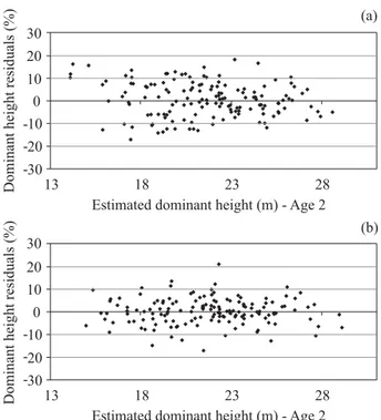
Thus, the tendency of precision improvement shown in the adjustment of the models was repeated in the validation process. The model considering climatic variables presented a gain of 19.8% in the dominant height estimate precision (as determined by the reduction in the standard error of estimate). The precision improvement was also verifi ed in the models’ relative residual plots, shown in Figure 1.
Table 4 – Adjustment statistics of the dominant height projection models.
Tabela 4 – Estatísticas de ajuste para os modelos de projeção da altura dominante.
Coeffi cient Parameter estimates Statistics
Wcv Climatic model Wcv Climatic model
A 35.503700 37.690300 R2 82.48% 88.74%
incl -0.211167 -0.215177 SEE 1.60m 1.26m
b1 0.015020 SEE% 7.28% 5.74%
b2 -0.035698
Wcv = Without climatic variables; SEE = standard error of estimate; SEE% = standard error of estimate in percentage
The residual plot without climatic variables (Figure 1a) showed a greater dispersion of the residuals when compared with the one with climatic variables, especially in the -10 to 10% of error range of younger dominant height projections (up to 20 meters). In the model with climatic variables (Figure 1b) the residuals tended to be more adherent to the zero value of the x-axis. Although slight, a visual reduction of the residual’s dispersion was observed in the model considering climatic variables, thus confi rming a greater stability of the adjustment and therefore better dominant height projection values. 3.3 Model sensibility
To test sensibility of the model to different climatic values input, a simulation was conducted considering different mean monthly precipitation amounts. All other variables were kept at constant values. The initial input values used were: Ag1 = 2.7; Ag2 = 5; Dh1= 15.4cm; radiation = 17.4MJ/m2/day; precipitation = 100mm/month. The monthly precipitation values used were correspondent to mean annual precipitation values ranging from 800 to 2300mm, with 500mm amplitude (Figure 2a). As for radiation the values ranged from 15.5 to 21.5MJ/m2/day, with 2MJ/m2/day amplitude (Figure 2b).
Figure 2a shows that dominant height growth is strongly affected by the precipitation regime in which it is inserted. This confi rms the fi ndings of Maestri (2003) and Temps (2005), who also found a strong correlation of dominant height growth and precipitation. At 800mm of mean annual precipitation, the projected value of the dominant height at age 5 years was 20.7m. In contrast, at 2300mm dominant height growth reached 29.1m, a 40% difference.
Solar radiation presented an inverse infl uence on dominant height growth (Figure 2b). The same behavior was found by Maestri (2003). This behavior can be Figure 1 – Dominant height relative residual plots of the models
without (a) and with (b) climatic variables using the validation data base.
attributed to a couple of factors. Firstly, radiation levels tend to be higher on dry seasons (BARRADAS, 1991; BROEK et al., 2001) when forest growth is reduced. Secondly, high incidence of solar radiation raises foliar temperature, which in turn raises foliar transpiration causing the tree to lose water to the environment and consequently grow less (KRAMER & KOZLOWSKI, 1960). The response of dominant height growth to different levels of solar radiation was weaker than the response to precipitation. At 15.5MJ/m2/day of mean daily radiation, the projected value of the dominant height at age 5 years was 23.8m. In contrast, at 21.5MJ/m2/day dominant height growth was reduced to 22.7m, a 5% difference.
4 CONCLUSIONS
The insertion of climatic variables (precipitation and solar radiation) in the inclination parameter of the Chapman and Richards’s model allowed for more precise dominant height projection estimates.
This methodology has its greatest application potential as a forest inventory data updater, in the sense that when past climatic history and stand condition is known, dominant height projection values can account for varying climatic conditions that affect forest growth.
Future projection values are limited by the lack of knowledge of future climatic conditions, however the knowledge of how Eucalyptus height growth varies
in relation to mean climatic conditions help predict productivity in areas without prior plantation history.
5 REFERENCES
ALMEIDA, A. C.; MAESTRI, R.; LANDSBERG, J. J.; SCOLFORO, J. R. S. Linking process-based and empirical forest models to use as a practical tool for decision-making in fast growing Eucalyptus plantation in Brazil. In: AMARO, A.; TOMÉ, M. (Ed.). Modelling forest systems. Walling Ford: CABI, 2002. p. 63-74.
BARRADAS, V. L. Radiation regime in a tropical dry deciduous forest in western Mexico. Theoretical and Applied Climatology, Amsterdam, v. 44, n. 1, p. 57-64, 1991.
BARROS, N. F.; SILVA, O. M.; PEREIRA, A. R.; BRAGA, J. M.; LUDWIG, A. Análise do crescimento de Eucalyptus saligna em solo de cerrado sob diferentes níveis de N. P. e K. no Vale do Jequitinhonha, MG. IPEF, Piracicaba, n. 26, p. 13-17, 1984.
BROEK, R. van den; VLEESHOUWER, L.; HOOGWIJK, M.; WIJK, A. van; TURKENBURG, W. The energy crop growth model SILVA: description and application to
eucalyptus plantations in Nicaragua. Biomass and Bioenergy, New York, v. 21, n. 5, p. 335-349, 2001.
CUNHA NETO, F. R.; SCOLFORO, J. R. S.; OLIVEIRA, A. D.; CALEGARIO, N.; KANEGAE JUNIOR, H. Uso da diferença algébrica para construção de curvas de índice de sítio para Eucalyptus grandis e Eucalyptus urophylla na região de Luiz Antonio, SP. Cerne, Lavras, v. 2, n. 1, p. 21-28, 1998.
Figure 2 – Dominant height projection estimates considering different mean annual precipitation (a) and solar radiation values (b).
KRAMER, P. J.; KOZLOWSKI, T. T. Physiology of trees. New York: McGraw-Hill Book, 1960. 642 p.
MAESTRI, R. Modelo de crescimento e produção para povoamentos clonais de Eucalyptus grandis considerando variáveis ambientais. 2003. 143 p. Tese (Doutorado em Ciências Florestais) - Universidade Federal do Paraná, Curitiba, 2003.
OLIVEIRA, A. D.; FERREIRA, T. C.; SCOLFORO, J. R. S.; MELLO, J. M.; REZENDE, J. L. P. Avaliação econômica de plantios de Eucalyptus grandis para a produção de celulose. Cerne, Lavras, v. 14, n. 1, p. 82-91, 2008.
SCOLFORO, J. R. S. Biometria fl orestal: modelos de crescimento e produção fl orestal. Lavras: UFLA/FAEPE, 2006. 393 p. (Textos Acadêmicos).
SCOLFORO, J. R. S. Biometria fl orestal: parte I, modelos de regressão linear e não-linear, parte II, modelos para relação hipsométrica, volume, afi lamento, e peso da matéria seca. Lavras: UFLA/FAEPE, 2005. 352 p. (Textos Acadêmicos).
SCOLFORO, J. R. S.; RIOS, M. S.; OLIVEIRA, A. D.; MELLO, J. M.; MAESTRI, R. Acuracidade de equações de afi lamento para representar o perfi l do fuste de Pinus elliotti. Cerne, Lavras, v. 4, n. 1, p. 100-122, 1998.
SNOWDON, P.; WOOLLONS, R. C.; BENSON, M. L. Incorporation of climatic indices into models of growth of Pinus radiata in a spacing experiment. New Forests, Netherlands, v. 16, p. 101-123, 1998.
TEMPS, M. Adição da precipitação pluviométrica na modelagem do crescimento e da produção fl orestal em povoamentos não desbastados de Pinus taeda L. 2005. 116 p. Dissertação (Mestrado em Ciências Florestais) - Universidade Federal do Paraná, Curitiba, 2005.
THIERSCH, C. R.; SCOLFORO, J. R. S.; OLIVEIRA, A. D.; MAESTRI, R.; REZENDE, G. D. S. P. Acurácia dos métodos para estimativa do volume comercial de clones de Eucalyptus sp. Cerne, Lavras, v. 12, n. 2, p. 167-181, 2006a.
THIERSCH, C. R.; SCOLFORO, J. R. S.; OLIVEIRA, A. D.; REZENDE, G. D. S. P.; MAESTRI, R. O uso de modelos matemáticos na estimativa da densidade básica da madeira em plantios de clones de Eucalyptus sp. Cerne, Lavras, v. 12, n. 3, p. 264-278, 2006b.