Testing the Optimality of Consumption
Decisions of the Representative
Household: Evidence from Brazil
*
Marcos Gesteira Costa
†
, Carlos Enrique Carrasco-Gutierrez
‡
Contents: 1. Introduction; 2. Method of Estimation; 3. Data; 4. Empirical Results; 5. Conclusion. Keywords: CCAPM, Rule of Thumb, Aggregate Consumption, Permanent Income Hypothesis, Euler
Equations. JEL Code: C32, E21.
This paper investigates whether there is a fraction of consumers that do not be-have as fully forward-looking optimal consumers in the Brazilian economy. The generalized method of moments technique was applied to nonlinear Euler equa-tions of the consumption-based capital assets model contemplating utility func-tions with time separability and non-separability. The results show that when the household utility function was modeled as constant relative risk aversion, external habits and Kreps–Porteus, estimates of the fraction of rule-of-thumb households was, respectively, 89%, 78% and 22%. According to this, a portion of disposable income goes to households who consume their current incomes in violation of the permanent income hypothesis.
Este artigo investiga se existe um comportamento subótimo nas decisões de consumo intertemporal na economia brasileira. O Método Generalizado de Momentos (MGM) foi aplicado ao modelo de precificação de ativos baseados no consumo (CCAPM) con-templando funções de utilidade separáveis e não separáveis. Os resultados mostram a existência de uma parcela da população que segue esse comportamento conhecido também como rule of thumb. Em termos mais concretos a fração de indivíduos que segue a regra de bolso é, respectivamente, de 89%, 78% e 22% para as funções de utilidade modeladas segundo as hipóteses de aversão relativa ao risco constante, há-bitos externos e Kreps–Porteus. De acordo com esses resultados, uma grande parcela da população consome totalmente a sua renda corrente o que implica em violação da hipótese da renda permanente.
*This article is a revised version of Marcos Gesteira’s Master Thesis, done under the supervision of Carlos Enrique Carrasco-Gutierrez. We gratefully acknowledge the comments and suggestions Fabio Reis Gomes, Wilfredo Maldonado, José Angelo Divino and seminar participants at UCB Brasília and Sociedade Brasileira de Econometria–SBE conference in Natal, 2014. We thank an anonymous referee and Alexandre B. Cunha (Editor) for the suggestions on an earlier version of this article. †Universidade Católica de Brasília, SGAN 916, Módulo B, Brasília, DF, Brasil. E-mail:[email protected]
1. INTRODUCTION
The permanent income hypothesis (PIH), described by Friedman (1957), states that transitory changes in income have little effect on consumer spending, while permanent income is responsible for most of the variation in consumption. In his seminal work, Hall (1978) founded a new approach to study aggregate consumption. By using Euler equations for the optimal choice of a representative consumer, he showed that consumption should follow a random walk and argued that this holds in empirical applications, for instance that postwar U.S. data are consistent with this implication. In contrast, Flavin (1981), using a rational expectations structure, argued that consumption is sensitive to current income and it is greater than that predicted by the permanent income hypothesis. This conclusion has been widely interpreted as evidence of the existence of liquidity constraint. Empirical evidence shows that liquidity constraint is one of the main reasons why it is difficult to observe consumption smoothing in the data. Based on this evidence, Campbell & Mankiw (1989, 1990) suggested that aggregated data on consumption would be better characterized if there were two types of consumers. They nested the PIH in a more general model in which a proportion λ of consumers follow the rule of thumb,1 consuming their current income (myopic spenders), while the remaining (1−λ)individuals consume optimally (optimizing savers). Using log-linearization of the model and instrumental variable estimates, they established by empirical application that there was a strong violation of the permanent income hypothesis because a significant fraction of the households have suboptimal behavior.
Cushing (1992) and Weber (2002) used intertemporally non-separable utility functions to study the behavior of American consumers. Cushing used a quadratic utility function modeled with current con-sumption and once-lagged concon-sumption. Weber (2002) generalized Cushing’s analysis by modeling the rule of thumb in nonlinear Euler equations and using the generalized method of moments (GMM) es-timation technique. In particular, he tested if the lifetime utility function is time non-separable and concluded that the effect of the rule of thumb was small and not statistically significant.
In this article, we follow the insight of Weber, who considered that consumption of the optimizing agent is aggregate consumption minus rule-of-thumb consumption. In addition, we use the consumption-based asset pricing model (CCAPM) of Breeden (1979) and Lucas (1978) as a base of modeling and testing. The CCAPM setup considers not only an interest rate as studied in Hall (1978), Flavin (1981), Campbell & Mankiw (1989) or Weber (2002), but several assets in the economy. For instance, Hansen & Singleton (1982, 1983) developed and tested the empirical implications of the PIH when asset returns are time-varying and stochastic. They used the S&P 500 index and Treasury Bill yield as a risk-free rates of return. Epstein & Zin (1991) used five individual stock return indexes which give value-weighted returns for broad groups of industrial stocks and Treasury Bill yields as a risk-free rates of return.
Regarding Brazilian data, some authors have tested the PIH by incorporating rule-of-thumb behavior, but no one has used this procedure of testing in the CCAPM setup2. Among the papers that have studied the rule-of-thumb proportion of consumption for the Brazilian economy are the articles of Cavalcanti (1993), Reis, lssler, Blanco, & de Carvalho (1998), Issler & Piqueira (2000), Gomes (2004) and Gomes & Paz (2004).
Cavalcanti (1993), studying the intertemporal elasticity of substitution with data from 1,980 to 1989, contemplated a budget constrained consumer in one of the models. He found that 32% of the population followed the rule of thumb. Reis et al. (1998), as Campbell & Mankiw (1989), used a model in which a portion of the population was restricted to consume only current income in order to test the validity of the PIH. Their study ranged from 1947 to 1994. The econometric tests revealed that about 80% of the population was restricted to consume only their current income. Issler & Piqueira (2000) conducted a study on the temporal series of consumption in Brazil from 1947 to 1994, aiming to examine theoretical
1These consumers are restricted to consuming their current income, with no optimizing behavior
issues of the PIH. The main results pointed to the acceptance of cointegration between consumption and income, and they also found that about 74% of the individuals are restricted in terms of liquidity. Gomes (2004) used Beveridge and Nelson’s decomposition to disclose a cyclical component in consumption when testing the PIH. When he adopted the habit formation specification he found similar results to those of Reis et al. (1998).
Gomes & Paz (2004) used panel data to test the applicability of the Keynesian theory, the PIH and the hybrid model to consumption decisions for Argentina, Brazil, Chile, Colombia, Peru, Paraguay and Uruguay. They used data from 1951 to 2000, and found values ofλthat ranged from 47% for Peru to 79% for Argentina. The fraction of Brazilian income that belongs to consumers constrained to spend their current income was 61% in their study. Arreaza (2000) examined wether liquidity constraints or voracity effects could explain consumption and saving in Latin America, using panel data from the period 1973 to 1993. She rejected the PIH, since around 20% of the consumption in Latin American follows predicted current income.
This article makes some contributions to the literature on aggregate consumption. First, we use a new procedure to test the rule-of-thumb behavior for Brazilian consumers. We use the consumption-based asset pricing model (CCAPM), which allows more than one interest rate. Second, this paper gen-eralizes the rule-of-thumb model to allow intertemporal non-separability in the representative house-hold’s preferences considering external habits (Abel, 1990). In addition, the Kreps–Porteus (Epstein & Zin, 1989, 1991) expected lifetime utility function, which separates the coefficient of relative risk aver-sion from the intertemporal elasticity of substitution, is employed. As complementary analysis, we study the traditional utility functional forms of constant relative risk aversion (CRRA). These different types of utility functions permit estimating the structural parameters: intertemporal discount factor, intertemporal elasticity of substitution, relative risk aversion coefficient and the habit formation param-eter. The purpose of this work is not to criticize the methods employed in previous articles, but instead to show a new procedure to test rule-of-thumb behavior for the Brazilian economy.
The empirical results in this paper provide evidences of rule-of-thumb behavior in the Brazilian case. In other words, there is a proportion of the individuals consuming their current income, and another group of individuals that consume optimally in each period. Therefore, there was a strong violation of the permanent income hypothesis.
The remainder of this paper is organized as follows. In section 2, the model with rule-of-thumb behavior is briefly discussed in the Euler equations for three different specifications. The estimation and results are detailed in section 3. Finally, the conclusions are in section 4.
2. METHOD OF ESTIMATION
2.1. Testing rule of thumb in the CCAPM framework
The idea behind the consumption-based capital assets model (CCAPM), established by Lucas (1978) and Breeden (1979), is that agents accumulate assets to ensure their future consumption plan, so the asset return series are related with the consumption series. The maximization problem faced by the agents is:
max [C2,t+s,θt+s+1]
∞
s=0
Ut(·) s.t.
C2,t+θt+1Pt=θtPt+θtdt+Yt
C2,t, θt+1≥0
andθ0is exogenous
, (1)
whereUt is the utility function in periodt;C2,t is the aggregated household’s consumption that
con-sumes according to optimizing behavior; θt is a vector of theN assets; Pt is the assets’ pricing
vec-tor for each period; and dt is the assets’ dividends vector.3 In each period, the agent receives an
3θ
tPt+θtdtis the total wealth the investor in periodt, also calledAt;θt+1Pt is the total wealth the investor will take from
exogenous income Yt, which is a state variable in the consumer problem. Solving this problem for
Ut= Et[∑∞s=0βsu(C2,t+s)]yields the Euler equations:
Pj,t= Et
[
β∂ut+1/∂C2,t+1 ∂ut/∂C2,t
(Pj,t+1+dj,t+1)
]
, forj= 1,2, . . . , N and ∀t, (2)
whereut(·)is the instantaneous utility function;βis the intertemporal discount coefficient; the index
j refer to each available asset, and
β∂ut+1/∂C2,t+1 ∂ut/∂C2,t
is the stochastic discount factor att+ 1. Dividing both sides byPj,t and placing the rights side under
(Pj,t+1+dj,t+1), it is possible to replace(Pj,t+1+dj,t+1)/Pj,t byRj,t+1, the gross return of assetjatt+1,
so that
1 = Et
[
β∂ut+1/∂C2,t+1
∂ut/∂C2,t Rj,t+1
]
forj= 1,2, . . . , N and ∀t. (3)
Hall (1978), using a quadratic utility functional form and fixed return rate, reached the conclusion that the aggregate consumption series behaves as a random walk:
∆C2
,t=ϵt, (4)
where∆C2
,tis the variation in consumption andϵt was called innovation. Campbell & Mankiw (1989)
divided consumers into two groups. The first group receives a share,λ, of the disposable income and consumes all their current income Y1,t; the second group receives a share (1−λ) of the disposable
income, follows the PIH and their income is Y2,t. Hence, the total income of the economy is Yt =
Y1,t+Y2,t, or
Yt=λYt+ (1−λ)Yt. (5)
The consumers from the first group have∆C1
,t=∆Y1,t=λ∆Yt, while the consumers from the second
group follow equation (4). The total variation in consumption can be stated as∆Ct =∆C1,t+∆C2,t, and replacing this yields Campbell and Mankiw’s test equation:
∆C
t=λ∆Yt+ (1−λ)ϵt. (6)
This equation says that the variation in consumption is a weighted average between the variation of the income of the first group and the unpredictable variation in the permanent income of the second group. They specified their hypotheses as
H0:∆Ct=ϵt, henceλ= 0
H1:∆Ct=∆Y1,t=λ∆Yt, henceλ >0.
(7)
Whenλ= 0, the permanent income hypothesis holds. Under the alternative hypothesis the change in consumption is a weighted average of changes in current income. Equation (6) should not be esti-mated by ordinary least squares (OLS) since the error component may be correlated with changes in income.
Weber (2002) modeled consumption in nonlinear Euler equations, by isolating the consumption of the second group,C2,t.4So, letCt=C1,t+C2,t, thenC2,t=Ct−C1,t, andC1,t=λYt, then
C2,t=Ct−λYt. (8)
4C
2,tis the consumption of the second group, optimizers. The consumers of the first group follow the rule of thumb, so their
The Euler equations of the CCAPM problem are only valid for optimizing consumers, replacing (8) in equation (3), and yields
Et
[
βu
′(
Ct+1−λYt+1)
u′(C
t−λYt) Rj,t+1
]
= 1 forj= 1,2, . . . , N and ∀t. (9)
Equation (9) can be used to estimate and to test the parameters of the model by the GMM technique. GMM estimators were developed by Peter Hansen in 1982. Since then this technique has enabled several breakthroughs in macroeconomics and finance research. The essence behind the GMM is to find a sample moment as close as possible to the population moment. Letθ˜be a vector of parameters andhanr×1 vector, where the lines are the orthogonality conditions. Thenθ˜satisfiesE[
h( ˜θ, wt)
]
= 0. In application with two assets’ returns, the number of orthogonality conditions arer= 2M, whereMis the number of instruments to be used in estimation. LetXtbe a vector of chosen instruments. Then the orthogonality
conditions are
h( ˜θ, wt) =
(
1−βu ′(
Ct+1−λYt+1)
u′(C
t−λYt) R1,t+1
) Xt
(
1−βu ′(
Ct+1−λYt+1)
u′(C
t−λYt) R2,t+1
) Xt
2M×1
. (10)
Therefore E[(1−βu ′(
Ct+1−λYt+1)
u′(C
t−λYt) Rj,t+1)
⊗Xt] = 0, for j = 1,2. The sample moment is defined as g( ˜θ, yt) = T1
∑T
t=1h( ˜θ, wt)and the GMM’s estimatorθ˜is the one that minimizes the scalarQ( ˜θ, yt) =
[g( ˜θ, yt)]′W[g( ˜θ, yt)], where W is the weighting matrix which acts to weight the various moment
conditions to build the distance measure.
A test for the over-identifying restrictions (TJ-test) allows checking whether the model’s moment conditions match the data well or not. The TJ statistic employed is asymptotically chi-squared with
r−k degrees of freedom, where r is the number of orthogonality conditions and k the number of parameters in the structural model.
2.2. Utility functions
The utility’s functional forms Constant Relative Risk Aversion Preferences (CRRA), external habits and Kreps–Porteus address time separability and non-separabibility.
The Constant Relative Risk Aversion Preferences
In the first model, the instantaneous utility funciton is parameterized as
u(C2,t) =
C21,t−γ−1
1−γ , and the utility funtionUtis
Ut= Et
∞ ∑
s=0
βsu(C2,t+s)
= Et
∞ ∑
s=0
βs
C21,t−+γs−1
1−γ
, (11)
whereγis the relative risk aversion coefficient and the reciprocal of the consumption’s intertemporal elasticity of substitutionψ= 1/γ.
The Euler equations are
1 = Et
[ β
( C2,t+1
C2,t
)−γ Rj,t+1
]
Replacing (8) in (12), yields
1 = Et
[ β
(
Ct+1−λYt+1
Ct−λYt
)−γ Rj,t+1
]
forj= 1,2, . . . , N and ∀t. (13)
Stationary regressors are obtained dividing throughCt, therefore
1 = Et
β
Ct+1
Ct −λ Yt+1
Ct
1−λYt Ct −γ
Rj,t+1
forj= 1,2, . . . , N and ∀t. (14)
LetXtbe a vector of chosen instruments, thus the orthogonality conditions are
E
1−β
Ct+1
Ct −λ Yt+1
Ct
1−λYt Ct −γ
Rj,t+1
⊗Xt
= 0 forj= 1,2, . . . , N and ∀t. (15)
The External Habits Preferences
This parametric form of the individual preferece assume that individual keeps the history of her own consumption, viewed as consumer’s habit, allowing for non-separability of the utility function over time. The instantaneous utility funciton for External Habits used is
u(C2,t, νt) =
[C2,t
νt
]1−γ
1−γ . Following Abel (1990), we specify the functionνt(·)here asνt=
[
C2D,t−1C1
−D
2,t−1
]κ
. In order to have “external habit”, we setD= 0andκ >0. Thereforeνt=
[ C2,t−1
]κ
and the utility funtionUt is
Ut= Et
∞ ∑ s=0
βsu(C2,t+s, νt+s−1)
= Et
∞ ∑ s=0 βs [
C2,t+s
(C2,t+s−1)
κ
]1−γ
1−γ
forj= 1,2,. . ., N and ∀t, (16)
whereC2,tis the individual consumption att;C2,t−1is the per capita aggregated consumption att−1;
κis a parameter controlling the time separability in the function. The Euler equations are
1 = Et
β ( C2,t+1
C2,t
)−γ( C2,t
C2,t−1
)κ(γ−1) Rj,t+1
forj= 1,2, . . . , N and
∀t. (17)
Replacing (8) in (17), yields
1 = Et
β (
Ct+1−λYt+1
Ct−λYt
)−γ(
Ct−λYt
Ct−1−λYt−1
)κ(γ−1) Rj,t+1
forj= 1,2, . . . , N and
∀t. (18)
Stationary regressors are obtained dividing throughCtandCt−1, therefore
1 = Et
β
Ct+1
Ct −λ Yt+1
Ct
1−λYt Ct
−γ Ct Ct−1
−λ Yt Ct−1
1−λYt−1
Ct−1
κ(γ−1)
Rj,t+1
Representing in the unconditional form, E
1−β
Ct+1
Ct −λ Yt+1
Ct
1−λYt Ct
−γ Ct Ct−1−λ
Yt Ct−1
1−λYt−1
Ct−1
κ(γ−1)
Rj,t+1
⊗Xt
= 0 forj= 1,2,. . .,N and ∀t. (20)
The Kreps–Porteus Preferences
The third utility preference treated here follow the Epstein & Zin (1989), being a generalization of the utility function proposed by Kreps & Porteus (1978). The aggregating function is parameterized as a constant elasticity of substitution (CES) function:
Ut=
[
(1−β)C2ρ
,t+β
(
EtU˜tα+1
)αρ] 1
ρ
, for0,ρ <1, (21)
whereEt is the conditional expectation operator given the information avaliable to the agent in the
planning period and U˜t+1 is the agent’s future utility. The consumption’s intertemporal elasticity of
substitution isψ= 1/(1−ρ). The relative risk aversion coefficientγis constant,γ= 1−α where the parameterα reflects the agent’s behavior towards risk. In particular, whenα= 0, we are back to the expected utility function with logarithmic preference. Whenα=ρ, we have and additively separable utility function.
The Euler equations are
1 = Et
β η ( C2,t+1
C2,t
)η(ρ−1)
˜
Bηt+1−1Rj,t+1
forj= 1,2, . . . , N and
∀t, (22)
whereη=α/ρandB˜
t+1is the optimum portfolio’s gross return.
Replacing (8) in (22) yields
1 = Et
β η (
Ct+1−λYt+1
Ct−λYt
)η(ρ−1)
˜
Bηt+1−1Rj,t+1
forj= 1,2, . . . , N and
∀t. (23)
Stationary regressors are obtained dividing throughCt, therefore
1 = Et
βη
Ct+1
Ct −λ Yt+1
Ct
1−λYt Ct
η(ρ−1)
˜
Bηt+1−1Rj,t+1
forj= 1,2, . . . , N and ∀t. (24)
In the unconditional form representation we have:
E
1−βη
Ct+1
Ct −λ Yt+1
Ct
1−λYt Ct
η(ρ−1)
˜
Bηt+1−1Rj,t+1
⊗Xt
= 0 forj= 1,2, . . . , N and ∀t. (25)
3. DATA
The series used for the estimation were the real per capita household consumption, real per capita gross domestic product (GDP), real gross returns of risky assets, and real gross returns of the riskless asset. The series of aggregate consumption, GDP and population are available at the website of IPEA (Instituto
de Pesquisa Economica Aplicada), while the series of return on assets and rates of inflation are posted at
The data range from 1995.Q1 to 2011.Q2. This period starts with the implementation of thePlano Real, the plan the Brazilian government launched that finally managed to end the persistently high in-flation (with bouts of hyperinin-flation) that had held sway over the previous two decades. Another factor that contributed to this choice was that Reis et al. (1998) and Gomes (2004) suggested that the high value ofλthey found was due to the credit constraint the Brazilian population encountered (high and unpre-dictable inflation with indexation not necessarily matched with salary indexation, making debt service as a proportion of household income extremely volatile). The lower inflation rates through the period studied in this paper resulted in credit expansion, the availability of funding to finance consumption was not at the same level as in the developed countries but was much higher than in the periods of the others studies. Therefore, a smaller part of the population following the rule of thumb was expected.
The series of the household consumption was calculated the same way as in Reis et al. (1998), where the gross fixed investment and current account balance series were subtracted from the GDP series to obtain a consumption of non-durable goods series.5
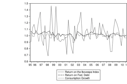
The returns of the IBOVESPA index were used to represent the returns of risky assets, because it is the most important index of average returns of the Brazilian stock market. Another interesting option would be IBrX, an index comprising more stocks that is widely used in the financial market for the static CAPM. However, the IBOVESPA series is longer and more suitable for the studied period. In order to represent the returns of the riskless asset in the Brazilian economy, the rate paid on government debt (SELIC rate) was used.6 The general price index (IGP-DI) calculated byFundação Getulio Vargas(FGV) was used to deflate income, consumption and returns of both assets. The consumption and income data were also subject to seasonal adjustments. Figura 1 shows the data in quarterly frequencies.
4. EMPIRICAL RESULTS
In this section, we present GMM estimates of the rule-of-thumb models for the utility preferences shown in the previous section. In order to estimate the orthogonality conditions, generated by the Euler
equa-Figure 1.Data on Quarterly Frequency (1995.Q1 to 2011.Q2).
0.6 0.7 0.8 0.9 1.0 1.1 1.2 1.3 1.4 1.5
95 96 97 98 99 00 01 02 03 04 05 06 07 08 09 10 11
Return on the Ibovespa Index Return on Fed. Debt Consumption Growth
5Income and consumption series were divided by the population series. Linear interpolation and extrapolation were applied to transform an annual population series into a quarterly basis series.
tions, we use several sets of instruments. The instruments correspond to lagged values of the growth in consumption and real interest rate.7 We also use the tests of the overidentifying restrictions (TJ-test) to assess the joint validity of each model and the set of instruments. In this paper, several sets of instruments were tested and none were rejected at the 5% level.
The results are presented in Tables 1, 2 and 3, where only display those where the parameter λ
estimate was between0and1.
For the CRRA utility, Tabela 1, the median estimate of the parameterλwasλˆ= 0.8945and all but
one of them were significant at the 5% level.
That is, results forλ show that around 89% of the population follows the rule of thumb. All the estimates of the intertemporal discount coefficient,β, were significant at the 5% level, and their median wasβˆ= 0.9783. The median for the relative risk aversion coefficient wasγˆ=−0.0974.
Tabela 2 reports the findings of the estimation of Euler equations (20) which correspond for the external habits utility model. Results show that overall estimations of the parameter λfor the most part were significant at the 5% level. The median of all valid estimates wasλˆ= 0.7817. It shows that
around 78% of the Brazilian population follows the rule of thumb. All the results for the intertemporal discount coefficient, β, were significant at the 5% level and their median wasβˆ = 0.9793. For the
parameter κ this study found κˆ = 0.1518, but only three of the estimates were significant at the 5% level. One positive feature of thisκ estimation is that it does not violate the external habit basic assumption: ifκ >0thanγ >0or ifκ <0thanγ <0. The relative risk aversion coefficient estimate wasγˆ= 0.0548and only four of them were significant at the 5% level and only one at the 10% level.
For the Kreps–Porteus utility function model, the findings for the estimation of the Euler equations (25) are shown in Tabela 3. We foundλˆ= 0.2263, but in almost all casesλestimates are not significant at
the 5% level. The intertemporal discount coefficient,β, was significant at the 5% level in 21 estimations, and the median of all estimations wasβˆ= 0.9743. Almost all the findings forη=α/ρwere very close
to zero,8however all the estimates, but one, were significantly different than zero. The median of all estimates was ηˆ = −0.00017, which yields αˆ = 0.00013and γˆ = 1.00013. For the parameterρ, six estimates were significant at the 5% level and the median of all estimates wasρˆ = 0.7721. The intertemporal elasticity of was captured by solving for each estimateψ= 1/(1−ρ)and the median of all estimates wasψˆ= 3.5798.9
In Tabela 4 we compare the estimates forβ,γandψwith studies that also used the CCAPM frame-work but did not contemplate the rule of thumb parameter in the model, such as Issler & Piqueira (2000), Bonomo & Domingues (2002), Catalão & Yoshino (2006).10 Tabela 4 shows the results of these studies forβ,γ andψ.
The results for the intertemporal discount coefficient,β, were all significant at the 5% level, for the three functional forms and in line with the previous studies.
Comparing the relative risk aversion results to the previous studies, we obtained lower values for the CRRA and the external habits utility models. Both models’ estimates were very close to zero. For the Kreps–Porteus utility function, the median of all estimates of the risk aversion parameter wasγˆ= 1.00013, in contrast what was found in Issler & Piqueiraγˆ= 0.68and Bonomo & Dominguesγˆ= 3.226. The intertemporal elasticity of substitution was captured by solving for each estimateψ = 1/(1−ρ) and the median of all estimates wasψˆ= 3.5798, while estimates by Issler & Piqueira, and Bonomo &
Domingues (2002) areψˆ= 0.29andψˆ= 0.371, respectively.
7A large number of instruments or a high number of assets can cause problems to find the optimal weighting matrix or influence the quality of asymptotic approximation, therefore the data must meet the following condition: N M(N M2 +1)< N T, whereN
are the number of Euler equations andTare the number of observations (Driscoll & Kraay, 1998). In this study, the number of instruments in the worst case the relation is78<122.
Table 1.Euler Equations for the CRRA Utility Function with Rule of Thumb.
E
1−β
Ct+1
Ct −λ Yt+1
Ct
1−λYt Ct
−γ
Rj,t+1
⊗Xt
= 0, forj= 1,2
whereN= 2,R1,t+1=Ibovespa returns, andR2,t+1=Returns on Selic.
Inst./Mtx β γ λ P(T-value×J)
I3/ASI 0.984*** 0.944 0.1530 0.414
(0.052) (0.7365) (1.1568)
I5/ASI 0.981*** 0.050 0.8049*** 0.462
(0.0035) (0.0517) (0.0246)
I1/NWFSI 0.974*** −0.974*** 0.8906*** 0.255
(0.0041) (0.0263) (0.0006)
I4/NWFSI 0.979*** −0.072 0.8945*** 0.806
(0.0029) (0.0435) (0.0099)
I3/NWFSI 0.978*** −0.138 0.8992*** 0.560
(0.0035) (0.1198) (0.0204)
I6/NWFSI 0.971*** −0.240 0.9522*** 0.252
(0.0032) (0.3293) (0.1109)
I4/NWVSI 0.969 −1.275*** 0.9853*** 0.991
(0.0004) (0.0572) (0.0042)
Median estimates 0.9783 −0.0974 0.8945 Confidence interval for the median:0.87≤λ≤0.915
Notes: (i) * , ** and *** denote, respectively, significance of parameter by thet-test at the 10%, 5% and 1% levels. (ii) The number in parentheses are the respective standard-deviation estimates, robust to heteroscedasticity and to serial correlation. (iii) The last line of the table shows the median of all estimates. (iv) List of instruments: I1 uses
R2,tR2,t−1,Ct/Ct−1,Ct−1/Ct−2; I3 usesR2,t−1,R2,t−2,Ct−1/Ct−2, andCt−2/Ct−3;
I4 uses R2,t−1,R2,t−2,R1,t−1,R1,t−2,Ct−1/Ct−2, andCt−2/Ct−3; I5 usesR1,t−1, R1,t−2,Ct−1/Ct−2, andCt−2/Ct−3; I6 usesR2,t,R2,t−1,R1,t,R1,t−1,Ct/Ct−1, and Ct−1/Ct−2. (v) The p-value of Hansen’s overidentifying restrictions test results are
Table 2. Euler Equations for the External Habits’ Utility Function with Rule of Thumb.
E
1−β
Ct+1
Ct −λ Yt+1
Ct
1−λYt Ct
−γ
Ct Ct−1−λ
Yt Ct−1
1−λYt−1
Ct−1
κ(γ−1) Rj,t+1
⊗Xt
= 0,forj= 1,2
whereN= 2,R1,t+1=Ibovespa returns, andR2,t+1=Returns on Gov.Debt-Selic.
Inst./Mtx β γ λ κ P(T-value×J)
I6/ASI 0.986*** 0.689** 0.122 0.582 0.398
(0.0031) (0.259) (0.5302) (0.4940)
I5/NWFSI 0.626*** 10.655** 0.419 1.6164*** 0.545
(0.2216) (5.0581) (0.2719) (0.4853)
I5/ASI 0.467*** 10.111*** 0.594** 1.280*** 0.784
(0.2111) (7.9961) (0.2240) (0.4685)
I4/ASI 0.977*** 0.067 0.769*** 0.1540 0.248
(0.0034) (0.0921) (0.0861) (0.1658)
I4/NWFSI 0.979*** 0.054 0.775*** 0.1517 0.497
(0.0021) (0.0632) (0.0644) (0.1245)
I8/NWFSI 0.978*** 0.035 0.7784*** 0.1978 0.149
(0.0034) (0.0734) (0.0594) (0.1711)
I7/NWFSI 0.979*** 0.011 0.7817*** 0.2008 0.550
(0.0033) (0.0906) (0.0813) (0.2471)
I6/NWVSI 0.977*** 0.120* 0.7956*** 0.0475 0.374
(0.0030) (0.0669) (0.0272) (0.0327)
I3/NWFSI 0.983*** 0.0579 0.7983*** 0.0065 0.542
(0.0031) (0.0523) (0.0355) (0.0214)
I3/ASI 0.981*** 0.0458 0.8063*** 0.0057 0.330
(0.0034) (0.0526) (0.0219) (0.0239)
I2/ASI 0.979 −0.065** 0.8905*** −0.0283** 0.284
(0.0048) (0.0272) (0.0008) (0.0134)
I2/NWFSI 0.972 −0.262 0.9177*** −0.1206 0.287
(0.0044) (0.3563) (0.0817) (0.1859)
Median estimates 0.9793 0.0548 0.7817 0.1518 Confidence interval for the median:0.717≤λ≤0.846
Notes:(i) * , ** and *** denote, respectively, significance of parameter by thet-test at the 10%, 5% and 1% levels. (ii) The number in parentheses are the respective standard-deviation estimates, robust to heteroscedasticity and to serial correlation. (iii) The last line of the table shows the median of all estimates. (iv) List of instruments: I2 usesR1,tR1,t−1,Ct/Ct−1,Ct−1/Ct−2; I3 usesR2,t−1,R2,t−2, Ct−1/Ct−2, andCt−2/Ct−3; I4 usesR2,t−1,R2,t−2,R1,t−1,R1,t−2,Ct−1/Ct−2, andCt−2/Ct−3; I5
usesR1,t−1,R1,t−2,Ct−1/Ct−2, andCt−2/Ct−3; I6 usesR2,t,R2,t−1,R1,t,R1,t−1,Ct/Ct−1, and Ct−1/Ct−2; I7 usesR2,t,R2,t−1,R2,t−2,R1,t,R1,t−1, andR1,t−2; I8 usesR2,t−2,R2,t−3,R1,t−2,
andR1,t−3. (v) Thep-value of Hansen’s overidentifying restrictions test results are shown in the last
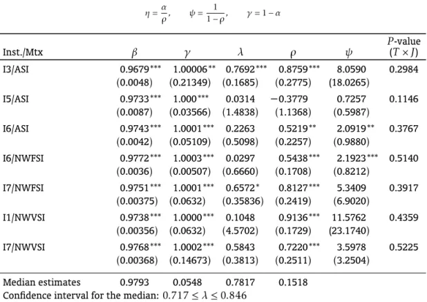
Table 3.Euler Equations for the Kreps–Porteus Utility Function with Rule of Thumb.
E
1−βη
Ct+1
Ct −λ Yt+1
Ct
1−λYt Ct
η(ρ−1)
˜
Bηt+1−1Rj,t+1
⊗Xt
= 0,forj= 1,2
whereN= 2,B˜t+1=Ibovespa returns,R2,t+1=Returns on Gov.Debt-Selic, and
η=α
ρ, ψ=
1
1−ρ, γ= 1−α
Inst./Mtx β γ λ ρ ψ P(T-value×J)
I3/ASI 0.9679*** 1.00006** 0.7692*** 0.8759*** 8.0590 0.2984
(0.0048) (0.21349) (0.1685) (0.2775) (18.0265)
I5/ASI 0.9733*** 1.000*** 0.0314 −0.3779 0.7257 0.1146
(0.0087) (0.03566) (1.4838) (1.1368) (0.5987)
I6/ASI 0.9743*** 1.0001*** 0.2263 0.5219** 2.0919** 0.3767
(0.0042) (0.05109) (0.5098) (0.2257) (0.9880)
I6/NWFSI 0.9772*** 1.0003*** 0.0297 0.5438*** 2.1923*** 0.5140
(0.0036) (0.00507) (0.6660) (0.1708) (0.8212)
I7/NWFSI 0.9751*** 1.0001*** 0.6572* 0.8127*** 5.3409 0.3917
(0.00375) (0.0632) (0.35836) (0.2419) (6.9020)
I1/NWVSI 0.9738*** 1.0000*** 0.1048 0.9136*** 11.5762 0.4359
(0.00356) (0.0632) (4.5702) (0.1729) (23.1740)
I7/NWVSI 0.9768*** 1.0002*** 0.5843 0.7220*** 3.5978 0.5225
(0.00368) (0.14673) (0.3813) (0.2511) (3.2504)
Median estimates 0.9793 0.0548 0.7817 0.1518
Confidence interval for the median:0.717≤λ≤0.846
Notes:(i) * , ** and *** denote, respectively, significance of parameter by thet-test at the 10%, 5% and 1% levels. (ii) The number in parentheses are the respective standard-deviation estimates, robust to heteroscedasticity and to serial corre-lation. (iii) The last line of the table shows the median of all estimates. (iv) List of instruments: I1 usesR2,t R2,t−1, Ct/Ct−1,Ct−1/Ct−2; I3 usesR2,t−1,R2,t−2,Ct−1/Ct−2, andCt−2/Ct−3; I5 usesR1,t−1,R1,t−2,Ct−1/Ct−2, and Ct−2/Ct−3; I6 usesR2,t,R2,t−1,R1,t,R1,t−1,Ct/Ct−1, andCt−1/Ct−2; I7 usesR2,t,R2,t−1,R2,t−2,R1,t,R1,t−1,
andR1,t−2. (v) Thep-value of Hansen’s overidentifying restrictions test results are shown in the last column. (vi) The
Table 4.Results of parametersβ,γ, andψin CCAPM studies.
β γ ψ= 1/γ
CRRA
This paper (with Rule of Thumb) 0.9783 −0.0974 −10.2669 Issler & Piqueira (2000) 0.99 0.62 1.61 Catalão & Yoshino (2006) 0.9711 2.1192 0.47 External Habits
This paper (with Rule of Thumb) 0.9793 0.0548 18.2482 Issler & Piqueira (2000) 0.99 0.46 2.17 Kreps–Porteus
This paper (with Rule of Thumb) 0.9743 1.00013 3.5798 Issler & Piqueira (2000) 0.96 0.68 0.29 Bonomo & Domingues (2002) 0.9505 3.23 0.37
Tabela 5 compares the results for the rule of thumb parameter with the previous findings with Brazil-ian data. The estimates for the CRRA and external habits were close to the findings of Reis et al. (1998), Issler & Piqueira (2000) and Gomes (2004), λˆ ≈0.80, λˆ ≈0.74 and λˆ ≈ 0.85 respectively. For the Kreps–Porteus model, the median estimate wasλˆ= 0.2263, but in almost all casesλestimates are not
significant at the 5% level. This number differs from the results for the two preference forms treated above and for the previous studies. If we took a different approach and considered only the results significant at the 5% level, the estimate for this parameter would beλˆ= 0.7692, very close to all the
other results.
For the CRRA and the external habits models, which yielded various significant results forλat the 5% level, we built confidence intervals. For the CRRA,[0.87,0.91]and for External habits,[0.72,0.85].
One possible reason pointed out for a highλ was the lack of credit available to the Brazilian pop-ulation during the period of study. After the end of the hyperinflation in 1994, the Brazilian economy experienced a strong expansion of credit, so some agents who followed the rule of thumb due to credit constraint in the previous studies could have started to optimize their consumption decisions.
Gomes & Paz (2004) and Arreaza (2000) results forλsuggests rejection of the PIH for Latin American data. This study comes to the same conclusion for Brazilian data, but reached to slightly different values for the fraction of myopic consumption.
Table 5. Results in the literature for the estimation of consumers’ share who follow the rule of thumb in the Brazilian economy.
Authors Period studied Estimates
Cavalcanti (1993) 1980 a 1989 0.32 Reis et al. (1998) 1947 a 1994 0.80 Issler & Piqueira (2000) 1947 a 1994 0.74
Gomes (2004) 1947 a 1999 0.85
Gomes & Paz (2004) 1951 a 2000 0.61
Gomes & Paz (2010) 1950 a 2003 [0.83,0.91](IPA)
[0.73,1.06](IGP-DI) This paper 1995 a 2011 [0.87,0.91](CRRA)
5. CONCLUSION
This paper investigated whether there is a fraction of consumers that do not behave as fully forward-looking optimal consumers in the Brazilian economy. We used different utility functional forms in the CCAPM framework. Beginning from Euler equations of the optimizing consumer utility problem, we estimated the structural parameters using the generalized method of moments (GMM) and tested the model’s over-identifying restrictions using Hansen’s TJ test (Hansen & Singleton, 1982).
Regarding the model’s performance, we conclude that in the Brazilian case there is a proportion of the individuals consuming their current income, and another group of individuals that consume opti-mally in each period. These findings suggest that a significant fraction of the Brazilian disposable income went to households who consumed their current income, following the rule of thumb. Therefore, there was a strong violation of the permanent income hypothesis.
The results found can be summarized as follows:
1. The main results show that for the CRRA and external habits utilities, most of the estimates of the rule-of-thumb parameters were statistically significant at conventional levels. The interval of confidence estimates results were[0.72,0.85]and[0.87,0.91]respectively.
2. For the Kreps–Porteus utility function almost all estimates of λwere statistically insignificant, therefore the 22% median estimate is not robust enough to say there was a fraction of myopic consumers.
3. The results for the intertemporal discount coefficient,β, were all significant at the 5% level, for the three functional forms and in line with the previous studies.
4. Comparing the relative risk aversion results to the previous studies, we obtained lower values for the CRRA and the external habits utility models.
There are two possible explanations of the higherλ reached in the present study. One possible reason for a high λ was the lack of credit available to the Brazilian population during the period of study. After the end of the hyperinflation in 1994, the Brazilian economy experienced strong expansion of the credit, so some agents who followed the rule of thumb due to credit constraint in the previous studies could have started to optimize their consumption decisions. On the other hand, the long period with no funds to finance consumption caused a large pent-up demand during the period of this study. Another explanation is that great increase in income experienced by the lower social classes, especially after 2002, caused them to increase spending in a Keynesian way, assuming that those social classes spend their current income.
Interesting extensions of this paper could be to use factor model analysis to build portfolios in order to consider more than two assets or to explore other functional forms.
REFERENCES
Abel, A. (1990). Asset prices under habit formation and catching up with the joneses.American Economic Review, 80(2), 38–42.
Andrews, D. W. K. (1991). Heteroskedasticity and autocorrelation consistent covariance matrix estimation. Econo-metrica,59(3), 817–858.
Arreaza, A. (2000, October 13). Liquidity constraints and excess sensitivity of consumption in Latin American
countries.Retrieved from http://www.cemla.org/red/papers2000/v_red_arreaza.pdf
Bonomo, M., & Domingues, G. (2002). Os puzzles invertidos no mercado brasileiro de ativos. In M. Bonomo (Ed.), Finanças aplicadas ao Brasil(pp. 105–120). Rio de Janeiro: FGV Editora.
Campbell, J. Y., & Mankiw, N. G. (1989, April).Consumption, income, and interest rates: Reinterpreting the time
series evidence(NBER Working Paper No. 2924). National Bureau of Economic Research. doi: 10.3386/w2924
Campbell, J. Y., & Mankiw, N. G. (1990). Permanent income, current income, and consumption.Journal of Business & Economic Statistics,8(3), 265–79.
Catalão, A. B., & Yoshino, J. A. (2006). Fator de desconto estocástico no mercado acionário brasileiro. Estudos
Econômicos,36(3), 435–463.
Cavalcanti, C. B. (1993). Intertemporal substitution in consumption: An empirical investigation for Brazil.
Brazil-ian Review of Econometrics,13(2), 203–229.
Cushing, M. J. (1992). Liquidity constraints and aggregate consumption behavior. Economic Inquiry,30(1), 134– 153. doi: 10.1111/j.1465-7295.1992.tb01540.x
Driscoll, J., & Kraay, A. (1998). Consistent covariance matrix estimation with spatially dependent panel data.
Review of Economics and Statistics,80(4), 549–560.
Epstein, L. G., & Zin, S. E. (1989). Substitution, risk aversion, and the temporal behavior of consumption and asset returns: A theoretical framework.Econometrica,57(4), 937–969.
Epstein, L. G., & Zin, S. E. (1991). Substitution, risk aversion, and the temporal behavior of consumption and asset returns: An empirical analysis.Journal of Political Economy,99(2), 263–286.
Flavin, M. A. (1981). The adjustment of consumption to changing expectations about future income. Journal of
Political Economy,89(5), 974–1009.
Friedman, M. (1957).A theory of consumption function. Princeton, NJ: Princeton University Press.
Gomes, F. A. R. (2004). Consumo no Brasil: Teoria da renda permanente, formação de hábito e restrição à liquidez.
Revista Brasileira de Economia,58(3), 381–402.
Gomes, F. A. R., & Paz, L. S. (2004). Especificações para a função consumo: Testes para países da América do Sul.
Pesquisa e Planejamento Econômico,34(1), 39–55.
Gomes, F. A. R., & Paz, L. S. (2010). Consumption in South America: Myopia or liquidity constraints. Economia
Aplicada,14(2), 129–145. doi: 10.1590/S1413-80502010000200001
Greene, W. H. (2008).Econometric analysis(6th ed.). Prentice Hall.
Hall, R. E. (1978). Stochastic implications of the Life Cycle-Permanent Income Hypothesis: Theory and evidence.
Journal of Political Economy,86(6), 971–87.
Hansen, L. P., & Singleton, K. J. (1982). Generalized instrumental variables estimation of nonlinear rational expec-tations models.Econometrica,50(5), 1269–1286. Retrieved from http://www.jstor.org/stable/1911873 Hansen, L. P., & Singleton, K. J. (1983). Stochastic consumption, risk aversion, and the temporal behavior of asset
returns.Journal of Political Economy,91(2), 249–265. Retrieved from http://www.jstor.org/stable/1832056 Issler, J. V., & Piqueira, N. S. (2000). Estimating relative risk aversion, the discount rate, and the intertemporal
elasticity of substitution in consumption for Brazil using three types of utility function.Brazilian Economic
Review of Econometrics,20(2), 201–239.
Kreps, D. M., & Porteus, E. L. (1978). Temporal resolution of uncertainty and dynamic choice theory.Econometrica, 46(1), 185–200.
Lucas, R. E., Jr. (1978). Asset prices in an exchange economy.Econometrica,46(6), 1429–45.
Newey, W. K., & West, K. D. (1987). A simple, positive semi-definite, heteroskedasticity and autocorrelation consis-tent covariance matrix.Econometrica,55(3), 703–08.
Newey, W. K., & West, K. D. (1994). Automatic lag selection in covariance matrix estimation.Review of Economic Studies,61(4), 631–654.
Reis, E., lssler, J. V., Blanco, F., & de Carvalho, L. M. (1998). Renda permanente e poupança precaucional: Evidências empíricas para o Brasil no passado recente.Pesquisa e Planejamento Econômico,28(2), 233–272. Weber, C. (2002). Intertemporal non-separability and “rule of thumb” consumption. Journal of Monetary