Simple tuning rules for deadtime compensation of stable, integrative, and unstable firstorder deadtime processes.

(1)

Simple Tuning Rules for Dead-Time Compensation of Stable,

Integrative, and Unstable First-Order Dead-Time Processes

Bismark C. Torrico,

*

,†

_{Marcos U. Cavalcante,}

†

_{Arthur P. S. Braga,}

†

_{Julio E. Normey-Rico,}

‡

and Alberto A. M. Albuquerque

†

Departamento de Engenharia Elétrica, Universidade Federal do Ceara, 60455-760 Fortaleza, CE, Braziĺ

‡

Departamento de Automacã̧o e Sistemas, Universidade Federal de Santa Catarina, 88040-900 Florianopolis, SC, Braziĺ

ABSTRACT: This work proposes a new and simple design for theﬁ_{ltered Smith predictor (FSP), which belongs to a class of}

dead-time compensators (DTCs) and allows the handling of stable, unstable, and integrative processes. For this purpose,ﬁ_{rst, to}

use lower-order controller andﬁ_{lters, it is shown that it is not necessary to use the integral action in the primary controller, which}

is used to tune the set-point response; then, the FSPﬁ_{lters are designed to obtain the desired disturbance rejection, robustness,}

and noise attenuation. Using this procedure, it is possible to obtain a better compromise between performance and complexity than other solutions in the literature. Two simulation case studies are used to compare the obtained solution with some recently published results. A practical experiment involving a neonatal intensive care unit is also presented to illustrate the usefulness of the proposed DTC.

1. INTRODUCTION

Dead-time processes are found in many industrial applications. Dead times are mainly caused by the time required to transport mass, energy, or information, but they can also be caused by processing time or by the accumulation of time lags in a number of simple dynamic systems connected in series.1−4

Conventional controllers such as proportional−integral−

derivative (PID) controllers can be used when the dead time is small, but they exhibit poor performance in the case of large dead times.5−7 _{The di}_ﬃ_{culties of controlling this type of}

process can be explained in the frequency domain: The dead time introduces a further decrease in the phase of the system that makes the process more diﬃ_{cult to control.}8 _{To solve}

these problems, dead-time compensators (DTCs) can be used.2 The Smith predictor (SP),9proposed in 1957, was theﬁ_rst

DTC strategy formulated to improve the performance of classical PI or PID controllers for processes with dead time. However, this strategy cannot be used in processes that have an unstable or integrative model, and its disturbance rejection response cannot be faster than the open-loop one.10 _Several

research studies involving attempts to overcome these diﬃ_{culties have been reported in the past 25 years.}2 _Two

main DTC groups have been received special attention from the academic community: DTC for integrative processes5,11−15

and DTC for unstable processes.16−19_{Wide reviews of these}

modiﬁ_{cations are presented in refs 2, 8, and 10. Uni}ﬁ_ed

solutions for dead-time processes, including robustness and disturbance rejection speciﬁ_{cations that can handle stable or}

unstable processes, were proposed in refs 20 and 21. However, these strategies have limitations in the case of unstable dead-time process with measurement noise. Despite the importance of noise, it was not a common practice to analyze noise eﬀ_ects

in previous DTC works. In dead-time process control, it is a common practice to use low-pass ﬁ_{lters as a unique tuning}

option to detune an initial controller setup to achieve loop requirements (robustness, sensitivity to noise, and so on). For

example, in refs 2 and 14, disturbance-observer dead-time compensators (DODTCs) andﬁ_{ltered Smith predictor (FSP)}

robustness ﬁ_{lters are presented; in ref 22, an internal model}

control (IMC) ﬁ_{lter was used, and in refs 20, 23, and 24,}

prediction errorﬁ_{lters were used. Nevertheless, in these works,}

noise ﬁ_{ltering was not studied. In a recent study,} 25 _{it was}

shown that previously cited works did not properly ﬁ_{lter the}

noise. To overcome this problem, the authors used an extra parameter in the FSP ﬁ_{lter, which increased the tuning}

complexity. In ref 26 was presented an applicable solution of the problems in refs 12 and 13 [known as the modiﬁ_{ed Smith}

predictor (MSP)] to control stable, integrative, and unstable dead-time processes, and it was shown that the MSP is a PID controller in series with a second-order ﬁ_{lter de}ﬁ_{ned by the}

dead time and an adjustable parameter. Nevertheless, an optimization tool is needed to set constraints on the robustness and sensitivity to measurement noise.

In this article, a simpliﬁ_{ed and new tuning procedure of the}

FSP for ﬁ_{rst-order stable, integrative, and unstable dead-time}

processes is proposed. It shown that, for these simple cases, it is not necessary to increase the order and complexity of the FSP

ﬁ_{lter to deal with the noise if the primary controller, used to}

tune the set-point response, is properly chosen. To illustrate this eﬀ_{ect, the proposed controller is tested in simulations and}

then for the temperature control of a neonatal incubator of the Electrical Engineering Department at the Federal University of Ceará, Fortaleza, Brazil.

The next section reviews the uniﬁ_{ed DTC approach, whereas}

section 3 describes the new simpliﬁ_{ed FSP tuning. Section 4}

presents two simulation case studies. An experimental case

Received: May 1, 2013

Revised: July 15, 2013

Accepted: July 25, 2013

Published: July 25, 2013

(2)

study is presented in section 5, and the work ends with some conclusions (section 6).

2. UNIFIED DTC APPROACH: A REVIEW

In this section, we summarize the ﬁ_{ltered Smith predictor}

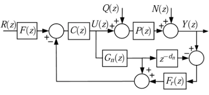
(FSP), which is one of the most popular DTC structures2,21,25 and can be used to control stable, unstable, and integrative dead-time processes. The FSP control structure is shown in Figure 1. As can be seen, the structure is the same as that of the

Smith predictor (SP) with two additional ﬁ_lters. _F₍_z_{) is a}

referenceﬁ_{lter to improve the set-point response, and}_F r(z) is a

predictorﬁ_{lter that improves the predictor properties, avoiding}

the appearance of slow or unstable poles of the plant in the disturbance rejection response and including extra parameters to improve robustness. In addition, Pn(z) = Gn(z)z−dn is the

nominal process discretized with a zero-order hold, where

Gn(z) is the dead-time-free model and dn is the nominal

discrete dead time. The equivalent control

two-degree-of-freedom (2DOF) structure for the FSP is shown in Figure 2, where

=

+ − −

C z F z C z

C z G z F z z

( ) ( ) ( )

1 ( ) ( )[1 ( ) d]

eq r

n r n (1)

=

F z F z

F z ( ) ( )

( ) eq

r (2)

Note thatCeq(z) must have at least one pole atz= 1 to reject

steplike disturbances and Feq(1) = 1 to guarantee set-point

tracking. In all previous works on FSP, this was achieved by using a pole at z = 1 in C(z), and the ﬁ_{lters were tuned to}

guarantee F(1) = 1 and Fr(1) = 1. In this article, we use a

simplerC(z) without a pole atz= 1 and lower-orderﬁ_{lters with} F(1) =Fr(1) =kr, wherekris a constant. Moreover, to obtain an

internally stable system,Ceq(z) cannot have zeros at the slow or

unstable poles of the plant.

Using the FSP structure, the nominal closed-loop transfer functions [whenPn(z) =P(z)] are

= =

+

H z Y z

R z

F z C z P z C z G z ( ) ( )

( )

( ) ( ) ( ) 1 ( ) ( )

yr n

n (3)

= = −

+

⎡

⎣

⎢ ⎤

⎦ ⎥

H z Y z

Q z P z

C z P z F z C z G z ( ) ( )

( ) ( ) 1

( ) ( ) ( ) 1 ( ) ( )

yq n n r

n (4)

= = −

+

H z U z

N z F z

C z C z G z ( ) ( )

( ) ( )

( ) 1 ( ) ( )

un r

n (5)

where R(z), Q(z), N(z), U(z), and Y(z) represent the z

transforms of the set point r(t), input disturbance q(t), measurement noisen(t), control signalu(t), and measurement outputy(t), respectively.

The implementation structure for unstable and integrative process, also called the uniﬁ_{ed dead-time compensator, is}

presented in Figure 3, whereS(z) is a stable transfer function computed with the equation21

= − −

S z( ) G z_n( )[1 z dnF z_r( )] ₍₆₎ Obtaining a stable function S(z) is equivalent to avoiding unstable pole−zero cancellations betweenCeq(z) andPn(z) or,

equivalently, having a stable function Hyq(z). The ﬁlter F(z)

and the primary controllerC(z) are used to obtain the desired set-point response, and Fr(z), which does not modify the

nominal set-point tracking, is used to the change disturbance rejection response and ﬁ_{lter the noise. Note that} _C₍_z_{) can}

increase the tuning diﬃ_{culty of} _F_r₍_z_{) because it a}ﬀ_{ects eqs 4}

and 5.

2.1. Tuning of the FSP.This subsection presents the main ideas and a brief analysis of the tuning procedure for the FSP presented in refs 2 and 25. The tuning of C(z) and F(z) is presentedﬁ_{rst, followed by the tuning of} _F

r(z).

2.1.1. Tuning of C(z) and F(z).AlthoughC(z) andF(z) are used to deﬁ_{ne the set-point response, it is important to notice}

thatC(z) also aﬀ_{ects the disturbance rejection (eq 4) and the}

noiseﬁ_{ltering (eq 5). Therefore, special attention must be paid}

to its tuning, mainly in the case of unstable processes. In refs 2, 21, and 25, C(z) and F(z) were designed using a traditional 2DOF approach. For example, in the case of aﬁ_{rst-order plus}

dead-time (FOPDT) model,C(z) is a PI controller, andF(z) is a ﬁ_rst-order ﬁ_lter.2 _{In general,} _F₍_z_{) is used to avoid the}

overshoot caused by the zeros introduced byC(z).

2.1.2. Tuning of Fr(z). Initially, the design of Fr(z) follows

two objectives: to decouple the disturbance rejection from the set-point response and to avoid the appearance of slow or unstable plant poles in the disturbance rejection response [giving an internally stable system whenP(z) is unstable].

Figure 1.FSP conceptual structure.

Figure 2.Two-degree-of-freedom (2DOF) structure.

(3)

To achieve this goal, consider the nominal model written explicitly in terms of numerators and denominators as in the equation

= − = ₋ ₊ −

P z N z

D z z

N z D z D z z ( ) ( ) ( ) ( ) ( ) ( ) d d n n n n n n n n (7)

where the roots ofDn+(z) are the undesired poles of the plant,

represented asDn+(z) = (z−z1)···(z−zn). The same is done

with the predictor ﬁ_{lter, which is written as}_F_r₍_z_{) = [}_N_r₍_z_)]/

[Dr(z)]. In ref 21, Fr(1) = 1 was considered. Thus, the ﬁrst

phase of the predictorﬁ_{lter design problem can be rewritten to} ﬁ_nd_N

r(z) in such a way that

− = −

= − − ··· −

− −

z F z D z z N z

D z

z z z z z z p z

D z z

1 ( ) ( ) ( )

( )

( )( ) ( ) ( )

( )

d d

d

r r r

r

0 1 n

r

n

n ₍₈₎

wherez0= 1 andp(z) is an unknown polynomial. Note that the

term (z−z0) appears only in the case thatC(z) has a pole atz

= 1. Thus, it will not appear in the simpliﬁ_{ed FSP (SFSP)}

proposed in this work. From eqs 8 and 6, we obtain

= ₋ −

S z N z D z

p z z z D z ( ) ( ) ( ) ( )( ) ( ) n n 0 r (9)

Now, S(z) is stable and does not have any of the undesired poles of Pn(z). As the roots of Dr(z) are poles of S(z) and Hyq(z), they deﬁne the disturbance rejection response and also

have connection with robustness. If desired, it is possible to obtain an ideal decoupling between the disturbance rejection and the step response. For this condition,Fr(z) should have fast

poles, andDr(z) andp(z) should be computed to eliminate the

poles ofHyr(z) fromHyq(z).21

2.2. Robustness and Stability Analysis.The robustness analysis was performed considering that the process modeling errors can be represented as unstructured uncertainties, that is,

P(z) = Pn(z) + ΔP(z) = Pn(z)[1 + δP(z)], where P(z)

represents the real process. Also, let us assume that an upper bound for the norm ofδ_P₍_z_),_z_{= e}jω′Ts for 0 < ω′<π_/_T_s_{, is}

given by δ_P_(ejω

′Ts_{). By de}ﬁ_nition, δ_P₍_z_{) is the norm-bound}

multiplicative uncertainty term, andTs is the sampling period.

In this case, consideringω₌ω′Ts, the robust stability condition

is22

δ ≤ = | + |

| |

ω ω

ω ω ω

P I C G

C G F

(e ) (e ) 1 (e ) (e ) (e ) (e ) (e )

j j

j j j

r n

n r (10)

where 0 <ω_<π_and_I r(ej

ω

) is deﬁ_{ned as the robustness index}

of the controller. Note that Dr(z) aﬀects the numerator of Ir(ejω), thus slow poles of Fr(z) give better robustness.

However, in the case of unstable processes, the robustness cannot be increased arbitrarily. This is an expected result because certain feedback action is needed to maintain stability and, thus, the detuning of the controller has a limit.21 Therefore, in practice, Fr(z) tuning is done to solve the

tradeoﬀ_{between robustness and disturbance rejection.}

3. NEW SIMPLIFIED FSP (SFSP) TUNING

This section presents a new simple method of tuning the FSP for stable, integrative, and unstable ﬁ_{rst-order plus dead-time}

(FOPDT) models. Consider the following FOPDT model

= =

−

− −

P z G z z b

z a z

( ) ( ) d d

n n 0

1

n n

(11)

To perform control tuning, it is assumed that the following speciﬁ_{cations are desired: (i) set-point following of steps with a}

deﬁ_{ned settling time, (ii) steady-state rejection of step}

disturbances with the same time constant as the set-point response, and (iii) noiseﬁ_{ltering and robust stability. Note that,}

in these speciﬁ_{cations, the same closed-loop time constant is}

deﬁ_{ned for all responses, which is a good solution in practical}

applications where robustness is an important issue.2

The tuning of the SFSP is performed in two steps: First,C(z) andF(z) are tuned for a desired step response, and then the

ﬁ_lter _F_r₍_z_{) is tuned considering both steplike disturbance}

rejection at steady state and the tradeoﬀ_{between robustness}

and disturbance rejection.

3.1. Tuning ofC₍z_{) and}F₍z_)._{Consider the desired} closed-loop transfer function

̅ = −

−

H z z

z z z ( ) (1 ) d

yr c

c

n

(12)

To achieve this objective, the primary controller and the referenceﬁ_{lter are proposed as}_C₍_z_{) =}_k_c_and_F₍_z_{) =}_k_r_{. Thus,}

usingkc,kr, and eq 11 in eq 3, we obtain

=

− +

−

H z k k b

z a k b z

( ) d

yr r c 0

1 c 0

n

(13)

Then, to makeH̅yr(z) =Hyr(z), the controller parameters must

bekc= (a1−zc)/b0andkr= (1−zc)/(a1− zc).

3.2. Tuning of the FilterF_r₍z_)._{For the proposed SFSP, the} ﬁ_lter _F_r₍_z_{) has three objectives: (i) to guarantee step}

disturbance rejection at steady state; (ii) to eliminate the open-loop pole fromHyq(z), which implies internal stability for

unstable plants; and (iii) to reach a compromise between robustness and disturbance rejection speed. To achieve these goals,ﬁ_{rst, the noise attenuation (eq 5) is rewritten using}_C₍_z₎

andF(z) from subsection 3.1 as

= − −

−

H z F z k z a

z z ( ) ( ) ( )

un r c 1

c (14)

As can be observed, aﬁ_{rst-order low-pass}ﬁ_{lter can be used to}

attenuate the noise at high frequencies. Nevertheless, to guarantee step input disturbance rejection and set-point tracking, a second-orderﬁ_{lter is used}14

α

= +

−

F z b z b z z ( ) ( ) r 1 2 2 2 (15)

whereb1andb2are used for theﬁrst two objectives andαfor

the third. To achieve objective i,Ceq(z) must have a pole atz=

1, and to achieve objective ii, the plant pole should not appear in the disturbance response, or equivalently, this pole should not be a zero ofCeq(z).

Using eq 1,Ceq(z) can be written as

=

−

+ −

⎡

⎣⎢ ⎤⎦⎥

C z F z

G z _{F z z}

( ) ( ) ( )

1

( ) C z G z

C z G z

d

eq r

n 1 ( ) ( ) ( ) ( ) r

n

n (16)

This implies that the term in the denominator of the second fraction on the right-hand side of eq 16, [1 + C(z) Gn(z)]/

[C(z)Gn(z)]−Fr(z)z−d, must be computed to cancel the plant

(4)

disturbance rejection of the system is that the same factor has a zero atz = 1.

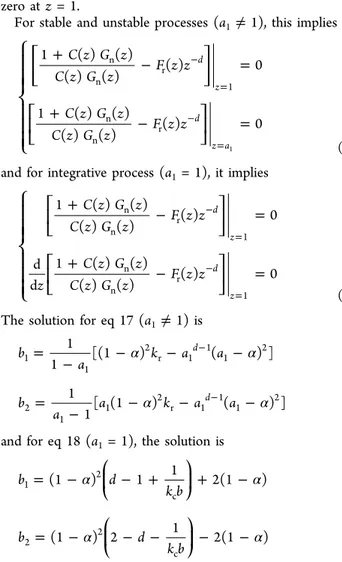
For stable and unstable processes (a1≠1), this implies

+ − = + − = − = − = ⎧ ⎨ ⎪ ⎪ ⎪ ⎩ ⎪ ⎪ ⎪ ⎡ ⎣ ⎢ ⎤ ⎦ ⎥ ⎡ ⎣ ⎢ ⎤ ⎦ ⎥ C z G z

C z G z F z z

C z G z

C z G z F z z 1 ( ) ( )

( ) ( ) ( ) 0

1 ( ) ( )

( ) ( ) ( ) 0

d

z

d

z a n

n r ₁

n

n r

1 (17)

and for integrative process (a1= 1), it implies

+ − = + − = − = − = ⎧ ⎨ ⎪ ⎪ ⎪ ⎩ ⎪ ⎪ ⎪ ⎡ ⎣ ⎢ ⎤ ⎦ ⎥ ⎡ ⎣ ⎢ ⎤ ⎦ ⎥ C z G z

C z G z F z z

z

C z G z

C z G z F z z 1 ( ) ( )

( ) ( ) ( ) 0

d d

1 ( ) ( )

( ) ( ) ( ) 0

d

z

d

z n

n r ₁

n

r

1 (18)

The solution for eq 17 (a1≠1) is

α α

=

− − − −

− b

a k a a

1

1 [(1 ) ( ) ]

d 1

1

2

r 1 1 1 2

α α

=

− − − −

− b

a a k a a

1

1[ (1 ) ( ) ]

d 2

1

1 2 r 1 1 1 2

and for eq 18 (a1= 1), the solution is

α α = − ⎛ − + + − ⎝ ⎜ ⎞ ⎠ ⎟ b d k b

(1 ) 1 1 2(1 )

1 2 c α α = − ⎛ − − − − ⎝ ⎜ ⎞ ⎠ ⎟ b d k b

(1 ) 2 1 2(1 )

2 2

c

whereα_{is the robustness tuning parameter. The SFSP can be}

implemented similarly to the FSP explained in the previous section.

3.3. Noise Attenuation Analysis.The worst case for the analysis of noise attenuation is the unstable case, where harder constraints are imposed onFr(z). Therefore, in this subsection

the noise attenuation is analyzed for this case. However, conceptually, the analysis is valid for the other cases as well. For simplicity, the following two assumptions are considered: (i)

Hun(ej

ω

) is analyzed atω₌π_{, because}_F_r_(ejω_{) is a low-pass}ﬁ_lter

and the noise can be interpreted as a high-frequency disturbance, and (ii)α_{tends toward 1 (}α_→_{1) to obtain the}

maximum attenuation bound ofFr(ejω) at ω= π. Thus, using

eqs 14 and 15 and the plant model, the bound of noise attenuation can be written as

̅ = | − − |

| + |

−

H a a a z

b z

( 1)( )

2 (1 ) d

un 1 1

12 1 c

0 c (19)

As can be observed, H̅undepends on the desired closed-loop

polezcand dead timed. To analyze the eﬀects ofzcanddon H̅un, H̅un was computed for several values of zc and d in the

ranges of [0.4−0.99] and [5−190], respectively, considering a plant withb0= 0.01 anda1= 1.01, as illustrated in Figure 4.

The following remarks are based on Figure 4: (i) Low values of

H̅unoccur in the region with high values ofzcand low values of dand (ii) high values ofH̅unoccur in the region with low values

ofzcand high values of d. In other words, a slow closed-loop

response and a short dead time contribute to better noise attenuation. Figure 5 shows numerical values of H̅un for

diﬀ_{erent values of} _z

c and d. As can be observed, for a given

value of H̅un, there is a limit on the achievable closed-loop

response (deﬁ_{ned by} _z

c) imposed by the dead time d: If the

dead time is large, then zc must be chosen high to keep the

desiredH̅unvalue. As theﬁlter cannot be tuned arbitrarily for a

desiredH̅unvalue, then special attention must be paid to the

desired closed-loop response by choosing an appropriate value ofzc.

4. SIMULATION CASE STUDIES

In this section, two case studies are presented, one for an unstable process and the other for an integrative process. The results obtained with the proposed SFSP are compared with those obtained with the FSP proposed in ref 25.

4.1. Unstable Process.The chemical reactor concentration control problem that was also used in refs 20, 21, and 25 is analyzed in this case study. This problem is used to show that correct tuning of the SFSP robustness ﬁ_{lter can e}ﬀ_ectively

reduce the eﬀ_{ect of noise, maintaining a good tradeo}ﬀ_between

robustness and performance. Moreover, a comparative analysis between the SFSP and FSP is presented. The linear concentration control process model is given by

=

−

− P s

s ( ) 3.433

101.1 1e s 20

(20)

The same sampling period as proposed in ref 20 was used here,

Ts = 0.5 s. Thus, the discrete model parameters are a1 =

1.00486,b0= 0.016689, andd= 40 (see eq 11).

Figure 4.Bound of noise attenuation|_H_̅_un|_{, three-dimensional plot.}

(5)

The FSP control parameters C(z), F(z), and Fr(z) were

deﬁ_{ned in ref 25 considering a closed-loop time constant of}τ₌

20 s and 30% dead-time estimation error as follows

= −

−

C z z

z ( ) 3.2501 0.98876

1 (21)

= −

−

F z z

z

( ) 0.4552 0.9753

0.98876 (22)

= −

− −

F z z z

z z

( ) 0.03535 ( 0.9968) ( 0.995)( 0.85) r

2

(23)

On the other hand, the proposed SFSP was tuned following the sequence of section 3. First, considering the same closed-loop time constant as used for the FSP, the primary control is

= − =

C z a z

b

( ) 1 c 1.7678

0 (24)

= −

− =

F z z

a z

( ) 1 c 0.83522

1 c (25)

wherezc= e−Ts/τ= 0.9753. Note that, if a faster or slower

set-point response is required, then the constant τ _{must be}

decreased or increased, respectively. Second, the robustness ﬁ_lter _F

r(z) is tuned based on 30%

dead-time estimation error by using α _{to satisfy the robust}

stability condition (see eq 10)

α

= +

− =

− −

F z b z b z z

z z z ( )

( ) 0.10204

( 0.99567) ( 0.977)

r 1

2 2

(26)

Note that b1 and b2 depend on α and the process model

parameters (see subsection 3.2). Observe thatα_{is the unique}

free tuning parameter ofFr(z) that can be tuned (i) with lower

values to obtain faster disturbance rejection and lower robustness or (ii) with higher values to obtain higher robustness but lower disturbance rejection.

Figure 6 shows the values of the robustness indexIr(ej

ω ) for both the FSP and the SFSP. A norm-bound multiplicative

uncertainty term, δ_P_(ejω

), deﬁ_{ned in subsection 2.2, is also}

depicted as a loop speciﬁ_{cation considering} ±_{30% dead-time}

estimation error. As can be observed, the SFSP has greater robustness than the FSP at midfrequencies, precisely where it is more important because the robustness stability condition (see eq 10) is closer to being violated.

In Figure 7, the noise attenuation|_H_un_(ejw₎_|_{is compared for} the FSP and SFSP. It can be observed that both controllers

attenuate the noise at high frequencies. Note that the FSP attenuates the noise more than the SFSP at high frequencies, which is an expected result because the order of the FSPﬁ_{lter is}

higher. Note also that the cutoﬀ_{frequency of the SFSP is at}

lower frequencies than that of the FSP.

To compare the performances of the FSP and SFSP, ﬁ_ve

scenarios of dead-time uncertainties were simulated: (i) 0% (nominal case), (ii) +30%, (iii) −30%, (iv) +60%, and (v)

−60%. In all ﬁ_{ve cases, a unity input step disturbance was}

added.

Figure 8 shows the closed-loop responses for the nominal case. In the same simulation, a measurement noise was added at

t = 600 s. The noise was generated by means of a Simulink band-limited white noise withTs= 0.5, noise power = 0.05, and

seed = 0. As can be seen, the SFSP rejected the disturbance faster than the FSP, and the two controllers attenuated the noise in similar ways.

Figure 9 shows the closed-loop response for the case with the dead-time estimation error of +30%. Note that the SFSP takes slightly longer to stabilize but its control signal is less oscillatory.

Figure 10 shows the closed-loop response for the case with the dead-time estimation error of −30%. Note that both the output and the control of the FSP are more oscillatory than those of the SFSP; in addition, the SFSP rejects the disturbance faster.

Figure 11 shows the closed-loop response for the case with the dead-time estimation error of +60%. Note that the FSP becomes unstable whereas the SFSP, despite a very oscillatory response, is stable.

Figure 6.Robustness index: Unstable plant.

Figure 7.Output−input noise gain.

(6)

Figure 12 shows the closed-loop response for the case with the dead-time estimation error of −60%. As can be seen, the proposed SFSP has a stable closed-loop response, and the FSP is unstable. (The FSP simulations were cut to obtain a clear

ﬁ_gure.)

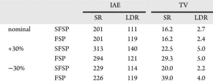
Finally, two performance criteria index were computed for both the set-point response (SR) and the load disturbance rejection (LDR): (i) the integrated absolute error (IAE) and (ii) the total variation of the input (TV).27 The results are presented in Table 1. Note the following points: (i) In the nominal case, the performances of the FSP and the SFSP are similar. (ii) In the case of the +30% dead-time estimation error, the FSP had a slightly better IAE; however, it had a worse TV for the SR. (iii) In the case of the−30% dead-time estimation error, the IAEs are similar for the two controllers; nevertheless, the proposed SFSP has a TV almost one-half that of the FSP. In

the cases of the ±60% dead-time estimation errors, the performance indices were not computed because the FSP had an unstable response.

4.2. Integrative Process. To show that the SFSP can handle integrative processes, we consider the process model presented in ref 23

=

+ + +

− P s

s s s s

( ) 0.1

( 1)(0.5 1)(0.1 1)e s 8

(27)

which is approximated by the following FOPDT model

= −

P s s

( ) 0.1e s

n 9.6 ₍₂₈₎

To design the controllers, the FOPDT model in eq 28 was discretized with a zero-order hold and a sampling time ofTs=

0.1 s.

The FSP and SFSP were tuned considering a dead-time uncertainty of±_{1 s and the di}ﬀ_{erence between}_P₍_s_{) and} _P_n₍_s₎

(eqs 27 and 28). Thus, for the FSP, the control parameters are

= −

−

C z z

z ( ) 11.4247 0.9714

1 (29)

= −

− F z z

z

( ) 0.5 0.9428

0.9714 (30)

= −

− −

F z z z

z z

( ) 0.0102 ( 0.9969) ( 0.995)( 0.92) r

2

(31)

and for the SFSP, they are =

F z( ) 1 (32)

=

C z( ) 5.7 (33)

Figure 9.System response with +30% dead-time error.

Figure 10.System response with−30% dead-time error.

Figure 11.System response with +60% dead-time error.

Figure 12.System response with−60% dead-time error.

Table 1. Performance Indices for the Unstable Examplea

IAE TV

SR LDR SR LDR nominal SFSP 201 111 16.2 2.7

FSP 201 119 16.2 2.4 +30% SFSP 313 140 22.5 5.0 FSP 294 121 29.3 5.0

−30% SFSP 229 114 20.0 2.2

FSP 226 119 39.0 4.0

a_{IAE, integrated absolute error; TV, total variation of the input; SR,}

(7)

= − −

F z z z

z

( ) 0.0553 ( 0.9964) ( 0.985)

r 2

(34)

Figure 13 shows the values of the robustness indexIr(ej

ω ) for both the FSP and the SFSP. In addition, the plant modeling

errorδ_P_(ejω_{) is depicted. Note that, as in the unstable case, the}

robustness index of the SFSP is larger than that of the FSP at the frequencies where the robust stability condition is closer to being violated.

To compare the performance between the FSP and the SFSP, three simulations were performed:ﬁ_{rst for the nominal}

case, second using the“real-plant”P(s) with 9 s of dead time, and third using the real-plantP(s) with some modeling errors that were not considered in the analysis.P(s) has 10 s of dead time and +10% error in the static gain and in the dominant time constant.

Figure 14 shows the simulation results for the nominal case. An input disturbance was applied at 30 s, and a measurement

noise was applied at 120 s. The noise was generated by means of a Simulink band-limited white noise with Ts = 0.1, noise

power = 0.01, and seed = 0. As can be observed, the SFSP rejected the input disturbance faster than the FSP, and the noiseﬁ_{ltering behaviors were similar.}

Figure 15 shows the results for the second case, for which the plant delay wasL= 9 s (see eq 27). An input disturbance was applied at 70 s. The FSP and SFSP had similar outputs for set-point tracking, although the FSP input was more oscillatory.

Regarding to input disturbance, the SFSP rejected it faster than the FSP.

Figure 16 shows the results for the third case, for which the errors in the static gain and dominant time constant of P(s)

were +10% and the dead time was 10. Note that the SFSP followed the reference and rejected the input disturbance whereas the FSP was unstable.

The integrated absolute error (IAE) and the total variation of the input (TV) were computed27 for both the set-point response (SR) and the load disturbance rejection (LDR). The results are presented in Table 2. Observe that (i) in the nominal case, the performances of both the FSP and SFSP were almost the same and (ii) in the case of L = 9 s, the two controllers had similar IAEs, but the proposed SFSP had a better TV. The performance indices were not computed for the other case because the FSP was unstable.

Figure 13.Robustness index: Integrative plant.

Figure 14.Nominal system response with disturbance and noise.

Figure 15.System system response if the real-plant dead time were 9

s.

Figure 16.Response if the real dead time were 10 s, with errors in the

static gain and dominant time constant of 10%.

Table 2. Performance Indices for the Integrative Examplea

IAE TV

SR LDR SR LDR nominal SFSP 10.7 12.1 5.7 1.1

FSP 10.7 14.5 5.7 1.1

L= 9 s SFSP 15 13.4 8.3 1.5 FSP 14.8 15.2 13.8 2.2

a_{IAE, integrated absolute error; TV, total variation of the input; SR,}

(8)

5. EXPERIMENTAL CASE STUDY

In this section, the SFSP algorithm is applied to control the temperature of a neonatal intensive care unit (NICU), shown in Figure 17, that belongs to the Electrical Engineering

Department of the Federal University of Ceará (Fortaleza, Brazil). A NICU is a device consisting of a rigid boxlike enclosure in which a newborn infant can be kept in a controlled environment for medical care. The incubator basically includes an ac-powered heater, a fan to circulate the warmed air, and transducers for relative humidity and temperature. Fresh air is driven by the fan toward the heating element, and then the warmed air goes into the NICU.

The control signal is measured in percentages in the range from 0% to 100%. The process variable is the temperature (in degrees Celsius) inside the NICU, which is the most important variable to be controlled. The model obtained using some step tests in the range of operation of the process and an oﬄ_ine

least-squares identiﬁ_{cation method is given by}

= −

− P z

z z

( ) 0.0018263 0.99337

30

(35)

where the sampling time was Ts = 0.4 min. To avoid

overheating next to the heater, the primary controller was tuned to have a safe closed-loop settling time of 1 h. Thus, the closed-loop pole was set tozc= 0.98, and aﬁlter withα= 0.93

was used to increase the robustness of the system and to attenuate the eﬀ_{ects of measurement noise.}

Figure 18 illustrates the experimental results obtained with the SFSP algorithm. Initially, the reference temperature (shown in dotted lines) was set to 32°_{C. At}_t_{= 120 min, the reference}

temperature was changed to 36°_{C. These reference values are}

commonly used in NICUs. It was observed that, for the two reference step changes, the overshoot was 0°_{C. Note that the}

overshoot was as expected, because, in section 3, it was designed to be zero. This is very important because it represents more comfort for the infant. To test the controller robustness, a disturbance was applied att= 260 min by opening two port holes of the NICU for 5 min. The port holes allow nurses and caretakers to handle the newborn without risk of contamination. Observe that there was an undershoot of 0.7

°_{C, but the temperature returned to the set point in 10 min.}

6. CONCLUSIONS

This article presents a new and simple design of the FSP called the SFSP that was specially designed for stable, integrative, and unstable FOPDT models. The algorithm uses a simple parameter to deﬁ_{ne the set-point following and two others to}

obtain the desired robustness and noiseﬁ_{ltering. This approach}

is simpler than those presented in refs 21 and 25, and the transfer functions of the SFSP are of lower order. The proposed SFSP presented good results in both simulated and practical experiments.

Two simulation cases were used to evaluate the robustness of the proposed SFSP. The SFSP presented a better robustness stability condition, a faster disturbance rejection, and a less oscillatory control signal even in the presence of dead-time error. These features are of interest for practical applications.

To evaluate the application of the SFSP algorithm to a real system, the problem of temperature control in a neonatal incubator was considered. The experiments showed responses with no overshoot and almost no oscillations of the control signal. Because of its simplicity and good performance, the SFSP presented in this work has great potential to be implemented in commercial neonatal intensive care units.

■

AUTHOR INFORMATION

Corresponding Author

*E-mail: bismark@dee.ufc.br. Tel.: +55-85-33669575. Fax: +55-85-33669574.

Notes

The authors declare no competingﬁ_{nancial interest.}

■

ACKNOWLEDGMENTS

Financial support from the Brazilian funding agencies CNPq and FUNCAP is gratefully acknowledged. The authors also thank the editor and anonymous reviewers for their suggestions and comments.

■

REFERENCES

(1) Marshall, J. E.; Górecki, H.; Walton, K.; Korytowski, A. Time-Delay Systems: Stability and Performance Criteria with Applications; Ellis Horwood: Chichester, U.K., 1992.

(2) Normey-Rico, J. E.; Camacho, E. F. Control of Dead-Time Processes; Springer: Berlin, 2007.

(3) Normey-Rico, J. E.; Camacho, E. F. Simple Robust Dead-Time Compensator for First-Order Plus Dead-Time Unstable Processes.Ind. Eng. Chem. Res.2008,47, 4784−4790.

Figure 17.Picture of the neonatal intensive care unit.

Figure 18. Experimental results of SFSP when controlling the

(9)

(4) Del-Muro-Cuéllar, B.; Valeco-Villa, M.; Jiménez-Ramírez, O.; Fernandez-Anaya, G.; Alvarez-Ramirez, J. Observer-Based Smith́

Prediction Scheme for Unstable Plus Time-Delay Processes. Ind. Eng. Chem. Res.2007,46, 4906−4913.

(5) Normey-Rico, J. E.; Camacho, E. F. A Unified Approach to Design Dead-Time Compensators for Stable and Integrative Processes with Dead-Time.IEEE Trans. Autom. Control2002,47, 299−305.

(6) Zhang, W. D.; Sun, Y. X. Modified Smith Predictor for Controlling Integrator/Time Delay Processes. Ind. Eng. Chem. Res.

1996,35, 2769−2772.

(7) García, P.; Santos, T.; Normey-Rico, J. E.; Albertos, P. Smith Predictor-Based Control Schemes for Dead-Time Unstable Cascade Processes.Ind. Eng. Chem. Res.2010,49, 11471−11481.

(8) Normey-Rico, J. E.; Camacho, E. F. Dead-Time Compensators: A Survey.Control Eng. Pract.2008,16, 407−428.

(9) Smith, O. J. M. Closed Control of Loops with Dead-Time.Chem. Eng. Progress1957,53, 217−219.

(10) Palmor, Z. J.The Control Handbook. Time-Delay Compensation: Smith Predictor and Its Modiﬁcations; CRC Press: Boca Raton, FL, 1996.

(11) Aström, K. J.; Hang, C. C.; Lim, B. C. A New Smith Predictor for Controlling a Process with an Integrator and Long Dead-Time.

IEEE Trans. Autom. Control1994,39, 343−345.

(12) Mataušek, M. R.; Micic, A. D. A Modified Smith Predictor foŕ

Controlling a Process with a Integrator and Long Dead-Time.IEEE Trans. Autom. Control1996,41, 1199−1203.

(13) Mataušek, M. R.; Micić, A. D. On the Modified Smith Predictor for Controlling a Process with a Integrator and Long Dead-Time.

IEEE Trans. Autom. Control1999,44, 1603−1606.

(14) Torrico, B. C.; Normey-Rico, J. E. 2DOF Discrete Dead-Time Compensators for Stable and Integrative Processes with Dead-Time.J. Process Control2005,15, 341−352.

(15) Watanabe, K.; Ito, M. A Process-Model Control for Linear Systems with Delay. IEEE Trans. Autom. Control 1981, 26, 1261−

1269.

(16) Liu, T.; Cai, Y. Z.; Gu, D. Y.; Zhang, W. D. New Modified Smith Predictor Scheme for Integrating and Unstable Processes with Time Delay.IEE Proc. Control Theory Appl.2005,152, 238−246.

(17) Lu, X.; Yang, Y.-S.; Wang, Q.-G.; Zheng, W.-X. A Double Two-Degree-of-Freedom Control Scheme for Improved Control of Unstable Delay Processes.J. Process Control2005,15, 605−614.

(18) Majhi, S.; Atherton, D. P. Modified Smith Predictor and Controller for Processes with Time-Delay.IEE Proc. Control Theory Appl.1999,146, 359−366.

(19) Tan, W.; Marquez, H. J.; Chen, T. IMC Design for Unstable Processes with Time-Delays.J. Process Control2003,13, 203−213.

(20) Albertos, P.; García, P. Robust Control Design for Long Time-Delay Systems.J. Process Control2009,19, 1640−1648.

(21) Normey-Rico, J. E.; Camacho, E. F. Unified Approach for Robust Dead-Time Compensator Design.J. Process Control2009,19, 38−47.

(22) Morari, M.; Zaﬁ_{riou, E.}_{Robust Process Control}_{; Prentice Hall:}

Upper Saddle River, NJ, 1989.

(23) García, P.; Albertos, P. A New Dead-Time Compensator to Control Stable and Integrating Processes with Long Dead-Time.

Automatica2008,44, 1062−1071.

(24) García, P.; Albertos, P.; Hagglund, T. Control of Unstable Non-Minimum-Phase Delayed Systems.J. Process Control2006,16, 1099−

1111.

(25) Santos, T. L. M.; Boutura, P. E. A.; Normey-Rico, J. E. Dealing with Noise in Unstable Dead-Time Process Control.J. Process Control

2010,20, 840−847.

(26) Matausek, M. R.; Ribič ́, A. I. Control of Stable, Integrating and Unstable Processes by the Modified Smith Predictor.J. Process Control

2012,22, 338−343.