Transactions of the VŠB – Technical University of Ostrava, Mechanical Series No. 1, 2011, vol. LVII
article No. 1860
Miluše VÍTEČKOVÁ*, Antonín VÍTEČEK**
COMPENSATION TUNING OF ANALOG AND DIGITAL CONTROLLERS FOR FIRST ORDER PLUS TIME DELAY PLANTS
KOMPENZAČNÍ SE ÍZENÍ ůNůLOGOVÝCH I ČÍSLICOVÝCH REGULÁTOR PRO
SOUSTůVY SE SETRVůČNOSTÍ PRVNÍHO ÁDU A DOPRůVNÍM ZPOŢD NÍM
Abstract
The article is devoted to the simple compensation tuning of analog and digital PI and PID con-trollers for the first order plus time delay plants. The described method makes controller tuning poss-ible so that the control process is non-oscillatory without an overshoot for all input variables. The use is shown in the example.
Abstrakt
Článek je v nován jednoduché kompenzační metod se ízení analogových i číslicových regulátor PI a PID pro proporcionální regulované soustavy se setrvačností prvního ádu a dopravním zpoţd ním. Popisovaná metoda umoţňuje se ízení regulátoru tak, aby regulační proces byl ne kmi-tavý a bez p ekmitu pro všechny vstupní veličiny. Pouţití je ukázáno na p íklad .
1 INTRODUCTION
Great attention is devoted all the time to PI and PID controller tuning. It is given in that indus-trial practice demands simple, reliable and at the same time robust controllers. Among these control-lers there belongs PI and PID controlcontrol-lers. Their operation is easily understandable and technical semi–skilled staff make up their tuning on the basis of the recommended methods. Unfortunately, at present there are a huge number of different kinds of controller tuning methods, in which the inexpe-rienced user is not oriented [1, 7, 8 – 10].
The described tuning method in the article is simple and relative robust. It enables analog and digital PI and PID controller tuning so that the control process will be non-oscillating without over-shoots. It is suitable for plants with the transfer function
s T
P d
s T
k s
G e
1 )
( 1
1
(1)
where k1 is the plant gain, T1– the time constant, Td – the time delay, s– the complex variable in the
L-transform.
It is supposed that the quantization error is negligibly small and therefore the terms discrete and digital can be considered as equivalent.
2 CONTROLLERS AND THEIR TUNING
The D-transform is used to have a uniform approach to analog and digital controllers. Detailed information about it can be found, e.g. in [2, 3, 6, 11, 12].
* Prof. Ing. Miluše VÍTEČKOVÁ, CSc., VŠB – Technical University of Ostrava, Faculty of Mechanical
Engineering, Department of Control Systems and Instrumentation, 17. listopadu 15, Ostrava – Poruba, 708 33, Czech Republic, tel. (+420) 59 732 4493, e-mail [email protected]
On the assumption that there is a D/A converter with the behavior of a sampler and a zero or-der holor-der, the plant D-transfer function has the form [11]
T T d a
T a T
ak
G T d
T d
P( ) 1 ( 1) , 1 e 1, (2)
where T is the sampling period, d – the relative discrete time delay (meanwhile the integer is sup-posed).
Further, the use of the standard controllers PI and PID are supposed, their transfer functions are given in Tab. 1 [11], where KP is the controller gain, TI – the integral time, TD – the derivative time, z– the complex variable in the Z-transform, γ– the complex variable in the D-transform.
Tab. 1 Transfer functions of standard PI and PID controllers.
L-transform Z-transform D-transform
PI
s T K
I
P 1 1
1 1
z z T
T K
I P
I P
T T
K 1 1
PID T s
s T
K D
I
P 1 1
z z T T z
z T
T
K D
I
P 1
1 1
1 1 1
T T T T
K D
I P
The compensation tuning of the PI and PID controllers is a very often used method in technic-al practice. It is given by its simplicity. The dynamic simplification is taken during the compensation and therefore it enables the use of analytical approaches.
The derivation procedure for computation of the adjustable controller parameters will be shown for the PID controller.
The D-transfer function of the PID controller with a cascade structure (with an interaction) has the form
) 1 (
] 1 ) ][( 1 ) [( 1
1 1 1 ) (
T T
T T T
T K T
T T
T K G
I
D I
P D
I P
C (3)
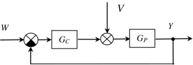
Consider the control system in Fig. 1, where W is the transform of the desired variable, v– the transform of the disturbance variable, Y– the transform of the controlled variable.
The open-loop D-transfer function on the basis of Fig. 1 for (2) and (3) can be determined
d
I
D I
P P
C
o T
a T T T
T T T
T K k G
G
G ( 1)
1 ) 1 (
] 1 ) ][( 1 ) [( )
( ) ( )
( 1 (4)
For the compensation it must hold
T a
a T T a T T
TI I
1 ) (
'* (5)
After the compensation the open-loop transfer function of the control system in Fig. 1 has the form
d I
D P
o T
T T
T T K k
G ( 1)
) 1 (
] 1 ) [( )
(
* 1
Fig. 1 Scheme of control system.
The controller gain KP* and the derivative time TD* can be determined by the multiple
domi-nant pole method (MDPM), which supposes that the essential behavior is given by a stable multiple dominant pole and influences of the non-dominant poles and zeros are negligible [4, 5, 11, 13].
The triple dominant pole 3*, the controller gain KP* and the derivative time TD* can be
ob-tained from three equations
0 d
) ( d , 0 d
) ( d , 0 )
( 2
2N N
N (7)
where the control system characteristic polynomial N(γ) can be determined from (6), i.e.
] 1 ) [( )
1 ( )
( 1 1 * T T
T K k T
N D
I P d
(8)
By solving the three equations (7) it is obtained
T T T
d d 2
2 )
2 (
2
*
3 (9)
d d
I P
d d d
a d a d
d T d
d T T K k
2 )
2 (
) 1 )( 1 ( 4 2 )
2 (
1 ) ( 4
2 2
* *
1 (10)
) ( 4 ) 1 ( 4 ) (
2 2
*
T T
T
d T d T T
d d
D (11)
The relations (5) and (9) – (11) directly hold for the PID digital controller with the cascade structure. For T→ 0 the corresponding relations for the PID analog controller with the cascade struc-ture can be obtained
d
T T
s lim 3* 2 0
* 3
d P
T P
T T T K k K
k * 2 1
1 0 * 1
e 4 )] ( [ lim ) 0
( (12)
1 * 0 *
) ( lim ) 0
( T T T
T I
T
I (13)
4 ) ( lim ) 0
( *
0
* d
D T D
T T T
T (14)
In relation (12) the equality
2 e 2 1 lim
d
d d
was used.
V
Y
P
G W
C
I D D I P C T T i T i T i T T i K
G , 1
) 1 ( 1 1 ) ( (15)
where i is the interaction factor.
For the PID controller with the parallel structure in accordance with (5), (10), (11) and (15) there is obtained
) 1 )( 1 ( 4 ) 1 )( 1 ( 4 ) ( ) ( 1 2 d a ad d a T T T T i I D (16) d P P d d d a ad d a i T K k T K k 2 ) 2 ( ) 1 )( 1 ( 4 ) ( ) ( 2 2 * 1 * 1 (17) T d a ad d a i T T T
TI I
) 1 ( 4 ) 1 )( 1 ( 4 ) ( ) ( 2 * * (18) T ad d a d a i T T T
TD D 2
2 * * ) 1 )( 1 ( 4 ) 1 ( ) ( ) ( (19)
The relations (17) – (19) directly hold for the PID digital controller with the parallel structure (Tab. 1). For T→ 0 the corresponding relations for the PID analog controller with the parallel struc-ture can be obtained (Tab. 1)
d d P T P T T T T K k K
k 1 * 12
0 * 1 e 4 )] ( [ lim ) 0 ( (20) 4 ) ( lim ) 0
( * 1
0 * d I T I T T T T T (21) d d D T D T T T T T T T 1 1 * 0 * 4 ) ( lim ) 0 ( (22)
The relations (17) – (19) for the PID digital controller with a parallel structure have unpleasant forms for practical use. They can be fundamentally simplified but it is somewhat inaccurate.
By the use of the first order Padé approximation, i.e. the approximate equality
2 1 2 1 e x x x (23)
in (5) it can be obtained
2 ) ( 1 * T T T
TI (24)
The approximation (24) for T1/T≥ 2 gives the error less than 3 % and for T1/T≥ 4 the error is
less then 1 %.
Similarly, by the use of the approximate equality (23) and the approximation
2
2 14 ( 1)e
1 2 ) 2 ( ) 1 ( d d d d d (25)
in (10) it is obtained
d P T T T T T K
k1 * 21 2
e ) e 14 ( ) 2 ( 2 ) ( (26)
The approximation (25) for d = T1/T≥ 2 gives the error less than 1 %.
The simplified relations for the PID digital controller with the parallel structure can be ob-tained from relations (16) – (19) after considering the approximation (23) – (26):
) 389 . 7 611 . 6 )( ( ) 2 )( ( 2 ] e ) e 14 )[( ( ) 2 )( (
2 1 2
2 2 2 1 * 1 d d d d d d d d P T T T T T T T T T T T T T T T T T T K
k (27)
) ( 4 ) 2 )( (
2 1 2
* T T T T T T T T d d d I (28) ] ) 2 )( ( 2 [ 2 ) 2 ( 2 1 2 1 * d d d D T T T T T T T T T (29)
The simplified relations are universal, for T > 0 hold for the standard PID digital controllers with the parallel structure and for T = 0 they hold for the standard PID analog controllers with the parallel structure.
By the similar approach after compensation accurate and simplified relations for the analog and digital PI controllers can be obtained.
The accurate relations are:
d P d d d a a T K k 1 ) 1 ( 1 ) ( * 1 (30) T a a T TI 1 ) ( * (31)
It can be easily shown that
d P T P T T T K k K k e )] ( [ lim ) 0
( 1 * 1
0 * 1 (32) 1 * 0 * ) ( lim ) 0
( T T T
T I
T
I (33)
For simplification of the relations (30) and (31) the approximation (23) and the approximate equality e ) 1 ( 4 1 1 1 1 d d d d d (34) were used.
The approximation (34) for d = Td/T≥ 1 gives the error less than 0.5 %.
The simplified relations for the computation of the adjustable parameters of the PI digital con-troller have the forms
d d P T T T T T T T T K k 437 . 5 563 . 2 2 ] e e) 4 [( 2
2 1 1
*
1 (35)
2
1
* T T
TI (36)
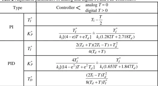
Tab. 2 Adjustable parameters of analog and digital PI and PID controllers.
Type Controller
<
analog T = 0 digital T > 0PI
*
I
T
2
1 T T
*
P
K
) 718 . 2 282 . 1 ( ] e e) 4
[( 1
*
1 *
d I
d I
T T
k
T T
T k
T
PID
*
I
T
) ( 4
) 2 )( (
2 1 2
T T
T T T T T
d
d d
*
P
K
) 847 . 1 653 . 1 ( ] e ) e 14 [(
4
1
*
2 2 1
*
d I
d I
T T
k
T T
T k
T
*
D
T *
2 1
) ( 8
) 2 (
I d
d
T T T
T T T
With respect to the compensation the described method is suitable for the FOPTD plants, for which inequality
d
T
T1 8 (37)
holds.
3 EXAMPLE
For the FOPTD plant with the L-transfer function
s P
s s
G e 6
1 6
1 ) (
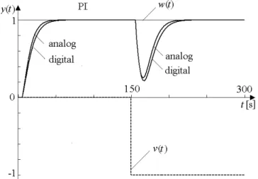
It is necessary to tune of the analog and digital PI and PID controllers so the servo and regulatory responses were non-oscillatory without overshoot. The time constant and the time delay are in seconds.
On the basis of Tab. 2 for k1 = 1, T1 = 6 sand Td = 6 sit is obtained:
PI controller
analog (T = 0): KP* 0.37; TI* 6
digital (T = 2): K*P 0.26; TI* 5
PID controller
analog (T = 0): K*P 0.68; TI* 7.5; TD* 1.2
digital (T = 2): K*P 0.43; TI* 6.13; TD* 0.92
Fig. 2 Responses of control system with PI controller.
Fig. 3 Responses of control system with a PID controller.
4 CONCLUSIONS
In this article the new compensation method for the tuning of analog and digital PI and PID controllers is described in detail. The method ensures the servo and regulatory responses non-oscillatory without overshoot. It is fully derived. Its use is easy and effective. In case of need the responses can be accelerated by increasing the controller gain.
This work was supported by research project GACR No 102/09/0894.
REFERENCES
[1] ÅSTRÖM K. J.
&
HÄGGLUND, T. Advanced PID Control. ISA – The Instrumentation, Systems, and Society, 460 pp., Research Triangle Park, 2006.[4] GÓRECKI, H. Analysis and Synthesis of Control Systems with Time Delay (in Polish). Wydawnictwo Naukowo – Techniczne, 372 pp., Warszawa, 1971.
[5] GÓRECKI, H., FUKSA, S., GRABOWSKI, P.
&
KORYTOWSKI, A. Analysis and Synthesis of Time Delay Systems. Polish Scientific Publishers – John Wiley & Sons, 369 pp., Warszawa-Chichester, 1989.[6] MIDDLETON, R. H.
&
GOODWIN, G. C. Digital Control and Estimation. A Unified Approach. Prentice-Hall, 1990.[7] O’DWYER, A. Handbook of PI and PID Controller Tuning Rules. 3rdEdition. Imperial College Press, 608 pp., London, 2009.
[8] SILVA, G. J., DATTA, A.
&
BHATTACHARYYA, S. P. PID Controllers for Time-Delay Systems. Birkhäuser, 330 pp., Boston, 2005.[9] VůŠEK, V., KOLOMůZNÍK, K.
&
JůNÁČOVÁ, D. Optimization and automatic control of chromium recycling technology,”. Proc. 5th WSEAS Int. Conf. on Simulation, modelling and optimization. Corfu, Greece, August 17-19, 2005, pp 391-394[10] VISIOLI, A. Practical PID Control. Springer-Verlag, 310 pp., London, 2006.
[11] VÍTEČKOVÁ, M.