Mutation load and the extinction of large populations

(1)

F_J_SEV1ER Physica A 230 (1996) 156-173

PHYSICA

Mutation load and the extinction of large

populations

A . T . B e m a r d e s 1

lnstitut ffir Theoretische Physik, Universitiit zu Krln, D-50923 Krln, Germany

Received 7 February 1996

Abstract

In the time evolution of finite populations, the accumulation of harmful mutations in further generations might lead to a temporal decay in the mean fitness of the whole population that, after sufficient time, would reduce population size and so lead to extinction. This joint action of mutation load and population reduction is called Mutational Meltdown and is usually considered only to occur in small asexual or very small sexual populations. However, the problem of extinction cannot be discussed in a proper way if one previously assumes the existence of an equilibrium state, as initially discussed in this paper. By performing simulations in a genetically inspired model for time-changing populations, we show that mutational meltdown also occurs in large asexual populations and that the mean time to extinction is a nonmonotonic function of the selection coefficient. The stochasticity of the extinction process is also discussed. The extinction of small sexual N ,-~ 700 populations is shown and our results confirm the assumption that the existence of recombination might be a powerful mechanism to avoid extinction.

1. Introduction

In the evolutionary process, deleterious mutations m a y arise when the genome o f one individual is formed. In an asexual population, assuming that there is no reverse mutations, these deleterious mutations will be transmitted to the descendents. For a sexual population the recombination process either can remove harmful mutations from the offspring's genome or can accumulate them in a higher rate. Moreover, new deleterious mutations m a y occur (independent o f the reproductive regime). One important question that arises in this context is: if we take into account the accumulation o f

1 Presently and permanently at Departamento de Fisica, Universidade Federal de Ouro Preto, Campus do Morro do Cruzeiro, 34500-000 Ouro Preto/MG, Brazil.

(2)

A.T. BernardeslPhysica A 230 (1996) 156-173 157

deleterious mutations from one generation to the following, is it possible that the progressive reduction of the fitness over several generations will cause the extinction of the species?

The discussion of different evolutionary scenarios produced by mutation (beneficial or detrimental), started in the 30s and one can observe a common feature through these decades: the assumption of an equilibrium state reached by the populations and their genome; or in the Haldane's [1] words: "abnormal 9enes are wiped out by natural selection at exactly the same rate as they are produced by mutation". This equilibrium state is reached asymptotically, as cited by Wright [2] when discussing the variation of gene frequency due to different causes. Based on the equilibrium assumption, Crow [3] discussed the genetic load of a population. Some analytical results have been obtained assuming very large or infinite population, an assumption that works together with that of the equilibrium state. One important traditional result is that the fitness of an infinite population is reduced by e - u , where U is the genome mutation rate. Discussing the mutation load in size varying (or small) populations, Kimura et al. [4] assumed Wright's distribution of gene frequency and observed that only for small populations

Neff

< 50 and higher selection was the mutation load higher than 1% (mutation load is the reduction of the population mean fitness due to the accumulation of harmful mutations). Reverse mutations have been considered, with a rate one order of magnitude below the forward rate. Comparing the incorporation of beneficial mutations between sexual and asexual populations, Crow and Kimura [5] showed that for small populations there is no important difference in the reproductive regime. Moreover, the advantage of recombination may be lost when an equilibrium state is reached. It is interesting to cite here the comparison between natural selection and classical mechanics done by Crow and Kimura [6]: natural selection has both the static and dynamical aspects. However, these dynamical aspects refer basically to the times before equilibration. Our question now is: what could be done if the attractor of a specific dynamics were the extinction of the population?

Obviously, if the equilibrium state is assumed, there is no way to answer properly the question of the extinction of a species addressed in the first paragraph. However, discussing the relation between recombination and mutation load, Muller [7] stated that for an asexual population a progressive genetic deterioration should be observed, with a progressive random loss of better fitted individuals, a process called by Felsenstein [8] "Muller's ratchet". Felsenstein noticed the discrepancy between results about the role of recombination, when infinite or finite population sizes had been assumed. The "Muller's ratchet" in selfing populations has been studied by Heller and Maynard Smith [9], who observed that for a large class of mildly deleterious mutations the ratchet mechanism is likely to be important.

(3)

158 A.T. Bernardes/Physica A 230 (1996) 156-173

Discrepancies between analytical and computer-simulated results can be observed in the work of Pamilo et al. [11], who pointed out that "discrepancy arises because the com- puter simulation allows a continuous accumulation of harmful mutations, whereas the

approximation used to derive Eq. (8) lead to a prediction o f a steady state". Lynch

and Gabriel [12] pointed out that the accumulation of deleterious mutations is expected to cause a gradual reduction in the population size down to zero, calling the syner- gistic interaction between fixation of harmful mutations and population reduction by "Mutational melt-down". The problems of Muller's ratchet operation and mutational meltdown are object of an increasing interest in the recent years [13-20]. One of the usual conclusions, confirming earlier assumptions, is that the extinction due to the fixation of detrimental mutations or loss of the better fitted individuals might be observed

in "small asexual populations or very small sexual populations with highly restricted

recombination or outcrossing" [15].

One important aspect of this mutational process is the evolution of senescence: natural selection will favour those genomes which accumulate mutations leading to detrimental effects at old ages [21 ]. In contrast with the results obtained with the steady-state assumption, Monte Carlo simulations on age-structured populations showed that mutational meltdown occurs even in large populations [22] (for a review of Monte Carlo simulations on biological ageing see [23]).

The aim of this paper is to study the time evolution of the populations away from equilibrium. In order to study this problem, we worked with computer simulation on a model introduced by Charlesworth [14]. Firstly, we are going to show that this model presents a scaling behaviour and that the basic assumption of fixed population cannot be considered as a general assumption. After that, as in previous work, we introduce a fixed population birth rate parameter allowing the time-changing of the population. Now we extend this previous study to a large range of selection values, discussing the role of slightly deleterious mutations. Environmental effects are also discussed. Moreover, we show that sexual reproduction can avoid the accumulation of harmful mutations.

2. Model

(4)

A.T. Bernardes/Physica A 230 (1996) 15~173 159 The evolutionary process is as follows: first we define an initial population and then mutation events take place. Thereafter one has the mating process and selection. After generating a population of N descendents the mutation process is resumed. In this part the population size is fixed and it will be changed below. Each combination of mutation, reproduction and selection represents one time step or one generation t. The mutations occur in loci selected at random in the entire genome and one assumes a Poisson distribution of mutation events with average rate mutr (typically we have used

mutr = 0.1, that means a mutation rate per locus

~10-4).

Back mutations are not accepted and if a selected locus has already a harmful mutation (bit--I), another one is chosen (this means that one has always 0 4 1 mutations).

In order to generate a zygote (an offspring), first one of the two chromosomes is drawn at random from a randomly selected individual and the number of crossovers

Nr is calculated, assuming a binomial distribution of recombination events with recombination rate per locus recr (typically recr = 0.0 - meaning no recombination; or recr = 0.001 - on average Nr = 1). By choosing at random these N~ crossovers locations, we recombine the two individual chromosomes (taking and linking parts of each one) and one has the first gamete (for more details see Ref. [24]). After that, the second gamete is generated: if Self = 1 this gamete will be drawn from the same parent and in the other extreme, for Self = 0, the second gamete is drawn from another parent chosen at random. For 0 < S e l f < 1 a random number between 0 and 1 is chosen and if this random number is larger than Self an outcrossing reproduction is assumed; otherwise, a selfing reproduction occurs. The second gamete is obtained by using the same recombination procedure described above. The "fusion" of these two gametes results in a zygote; in our picture two new sets of computer words.

The fitness of this new zygote is computed as follows. When one gene occurs in dissimilar allelic forms at a specific locus it is called heterozygous; otherwise it is called homozygous. One assumes that the fitness f of the unmutated genotype is f = 1 and, by introducing one harmful mutation in the genotype, its fitness will decrease by a factor of (1 - s) in the case of homozygous mutations or (1 - hs)

for heterozygous, s being the coefficient o f selection and h the dominance coeffi- cient. In the example shown below, an individual has 2 heterozygous alleles (loci 2 and 8) and 2 homozygous harmful alleles (loci 5 and 12) in the first 16 loci of its genome:

b i t ( l o c u s ) 1 2 3 4 5 6 7 8 9 10 11 12 13 14 15 16 chrom. 1 0 1 0 0 1 0 0 0 0 0 0 1 0 0 0 0 chrom. 1' 0 0 0 0 1 0 0 1 0 0 0 1 0 0 0 0

(5)

160 A. T. Bernardes / Physica A 230 (1996) 156-173

given by

f = (1 - s)U(1 - h s ) °. (1)

If the fitness is less than a random number (0,1), the zygote is rejected; otherwise it is accepted and the entire process is resumed until one has a number of surviving zygotes equal to N. Thus, the total population remains constant during the simulation. After reproduction-selection is finished, the zygote population substitutes the old individuals and therefore there is no overlap between the populations. New mutations occur and this process continues through the generations.

As one can see below, for several sets of parameters the mean fitness of the N individuals decays so that in later generation one needs to produce more zygotes than in the earlier. Since one needs to create more and more descendants generation after generation, this model has an increasing time-dependent birth rate. In later papers, Charlesworth et al. [15, 16] observed that the fitness depends on the initial size of the population: the larger N is the slower the fitness decreases. Thus, they state that the problem of extinction arises only in small asexual population (or in very small outcrossing populations), when the fitness decreases fast. Similar statements can be observed in other papers.

3. Results and discussions for fixed populations

(6)

A.T. BernardeslPhysica A 230 (1996) 156-173 161

(D ¢/) 03 I t .

0.95

0.90

0.85

0.80

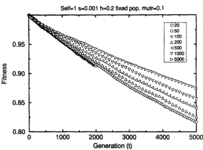
Self=l s=0.001 h=0.2 fixed pop. mutr=0.1 • i • i • i - i •

~ : ~ , ~ , < ~ < f v v w v~,~,~,~

",<~b-..,~ A ^ "q<1~ V v ~ ~ " G ~ / ~ A ~ "~<I<~ <~ vv~7~;

o<

i I , I i I i I *

0 1000 2000 3000 4000 5000

Generation (t)

Fig. 1. Population mean fitness versus generation in selfing populations Self=l obtained for different population sizes (provided in the figure legend) under multiplicative selection. The results were averaged over 20 samples. The simulations started with mutation-free genome. The selection coefficient is s = 0.001, dominance coefficient h = 0.2, recombination rate recr = 0.0 and mutation rate mutr = 0.1.

o f ~:

S ~ t

0.001 0.12 0.005 0.23 0.01 0.38 0.02 0.72

(7)

162 A.T. BernardeslPhysica A 230 (1996) 156-173

U'J

C

u .

1.00

0.90

0.80

0.70

0 10000

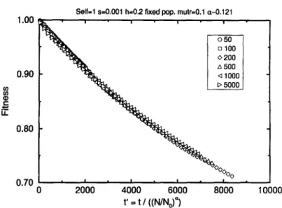
Self=l s=0.001 h=0.2 fixed pop. mutr=0.1 a-0.121

%

I a I m I = I =

2000 4000 6000 8000

t' = t / ((N/No) ~)

Fig. 2. Time scaling of the population mean fitness presented in Fig. 1. Here the time for each generation

was divided by the factor (Ni/No) ~ where No = 50, with the values of Ni being shown in the legend. Note

that all the curves overlap with that for No = 50.

L L 0.90

0.80

0.70

0.60

0.50

0.40 0

Self=l h=0.2 fixed pop. N=50 mutr=0.1

O O " u •

~ - l l ~ ; . - u 1 3 o - - ~ O O c x ) c ' v - ~ . . . . d l "..~9 O O ~ " - ' ~ u u O O C x 3 C

•

~ _

aaa

a

~Z~

% o

~°°°~o

v--

v

oo.oo51 ~=

% 0

®~c

oo.o~ I "%~^

%00

z~0.o2 ]

W~I~,,

00%

• ,=0.05 I ' ~

ooo¢,^

VO.I I ,,, v %

• 0.2 I ~,t~. 0 0 0 ¢

• o.3 I ~ ¢'

1000 2000

Generation (t)

Fig. 3. Population mean fitness versus generation in selfing populations Self----1 obtained for different selection

coefficient s (shown in the figure legend). Multiplicative selection has been assumed and the simulations have been performed for a fixed population of N = 50 individuals. The results were averaged over 20 samples (s ~< 0.02) and 30 samples (s >/0.05). The other parameters are the same as described in Fig. 1.

(8)

A.T. Bernardes/Physica A 230 (1996) 156-173 163

0.90

0.70 o

u_

0 . 5 0

Self=l h=0.2 fixed pop. N=50 mutr=0.1 "

~Jl.~ % ,%%

NN %111

\ \

\ k I I

",,

, ,,

\ \ I I

\ I

I

\ I

\ !

0 . 3 0 . . . 1 0 "4 1 0 -3 1 0 "2 1 0 - I

s e l e c t i o n s

Fig. 4. Fitness values at different times: t = 1000 and 2000 (provided in the legend) obtained from the curves shown in Fig. 3. Here the nonmonotonic dependence of the fitness on the selection coefficient is clearly observed: for higher or lower values of s the fitness increases. The dashed curves are provided as a guide.

Selling fixed population (Self=l)

1 . 0 0 • • • , - • • 1 . 0 0

0 1000 2000

Generation (t) 0.60

u_

0.60

0 . 8 0

0.60

Outerossing fixed population (Self=O) gO^' " " ' "

i!! 1

oo. o ° ~

ooooM~-I¢

e e e

!

0 1000 2000

Generation (t)

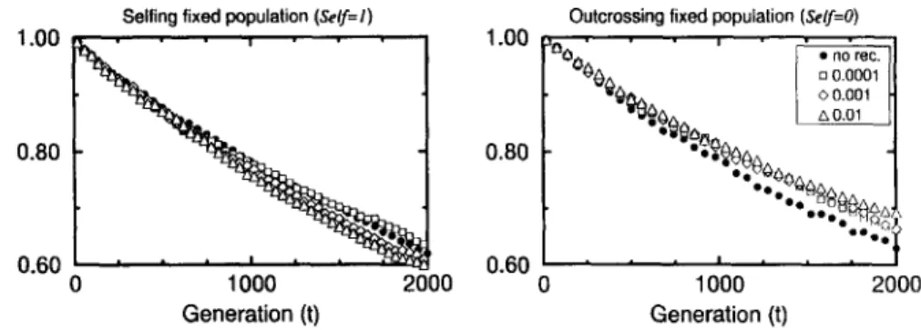
Fig. 5. Population mean fitness versus generation in asexual (left) and sexual (right) populations obtained for different recombinations (provided in the legend). A fixed population of N = 100 individuals has been used. All the simulations started with no mutation. The selection coefficient is s = 0.01, dominance coefficient

h = 0.2 and mutation rate mutr = 0.1. The results were averaged over 10 samples.

reached), the e q u i l i b r i u m a s s u m p t i o n c a n n o t be a s s u m e d a priori, due to the fact that, b y c h a n g i n g some parameters, the b e h a v i o u r o f the system might be u n k n o w n .

(9)

164 A.T. Bernardes/Physica A 230 (1996.) 156-173

cases without recombination are shown with filled circles whilst the open symbols are related with different recombination rates (provided in the legend). Here we have used a fixed population of N = 100 individuals and the other parameters are the same as cited above. For outcrossing populations it is clearly seen that the introduction of the recombination compared to the case without recombination increases the population mean fitness. Moreover, the higher recr is, the slower the fitness decays. Once again, fitness always shows a constant decay with time, even for the highest value of the recombination rate (recr = 0.01). For selfing populations, a slight increase in the fitness is observed when a low recombination rate is assumed (recr = 0.0001). However, the fitness decreases for higher values of recr. Our suspicion is that in this case the recombination process might be increasing the accumulation of deleterious mutations. If one compares the fitness for selfing and outcrossing populations, in contrast with the results obtained for higher s, now the better fitness has been obtained for outcrossing populations, though they are not too different.

At this point, we summarize the results obtained taking into account the fixed population assumption. This model shows two different scaling behaviours: a power-law scaling for weak selection and a exponential scaling for strong selection. It means that this system never reaches the equilibrium state and the equilibrium assumption cannot be assumed a priori. Under strong selection it has been shown that the recombination produces better results for selfing populations and now we showed that for weak selection the contrary occurs, though the increase for outcrossing populations does not allow one to assume that it might avoid a constant deterioration of the species. Moreover, for selfing populations under weak selection it is not clear the role of the recombination process. In the next section we shall describe the results obtained using a time-changing population.

4. Time-changing populations: evolution out of the equilibrium

To simulate a changing population, two new parameters have been introduced in the model. The first parameter represents the reproductive rate Birth, i.e., the total population can grow by the expression: N ( t + 1) = Birth × N ( t ) . To prevent the population

(10)

A. T. Bernardesl Phy sica A 230 (1996) 156- l 73 165 zyxwvutsrqponmlkjihgfedcbaZYXWVUTSRQPONMLKJIHGFEDCBA

Self=1 ~~0.01 h-0.2 N(O)=50 mulb0.1 zyxwvutsrqponmlkjihgfedcbaZYXWVUTSRQPONMLKJIHGFEDCBA

I I I I

q onmnDolll

Generation (t) Generation (t)

0.8

1

o1,ooo

A5.000 D 10,000 v 50,000 OlOO,Mx1

q 5ooOa

L

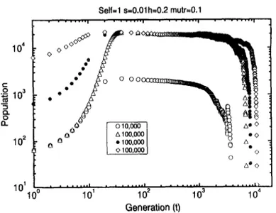
Fig. 6. Time evolution of the population (left) and population mean fitness (right) for selfing Self=1 populations under multiplicative selection obtained for initial population N(0) = 50 and different environmental carrying capacities Nmar (provided in the figure). No recombination has been assumed. The general parameters are: s = 0.01, h = 0.2 and MU@ = 0.1. For N mar < 10 000 the results were averaged over 20 samples while for Nmar > 50 000 the result obtained for just one sample is shown.

not survive. However, it is not substituted by another trial (as one has been done to the fixed population case). The population at generation (t + 1) is formed by those zygotes which survive at time t.

In the following, we are going to show the results obtained taking into account different situations. All the results were averaged over several samples, though very large simulations represent just one sample (cited in the figure captions). When an extinction was observed (in the case of parallel run), the quantities of interest were averaged only over the remaining samples.

4.1. The eflect of environmental carry ing capacity

In Fig. 6 we show the results obtained for a selfing population without recombination. The initial population is N(0) = 50 individuals, with Birth = 1.3 and different environmental carrying capacities NmM were used (the values are provided in the legend). In these results we have assumed: selection coefficient s = 0.01, dominance coefficient h = 0.2, mutation rate mutr = 0.1. The evolution of the total population (at left) and the population mean fitness (at right) are shown. Initially, the population grows, attain- ing a maximum value imposed by the environmental carrying capacity. A further slow decline in the population size can be observed, due to the fact that more and more zygotes do not survive. This corresponds to the decay in the population mean fitness, as one can observe in the right plot. Finally (except for the largest Nmar), the population extincts. Thus, the reduction of the population mean fitness leads to a reduction in the population size. Even for N,, = 500000 a slight decline in the population mean fitness is observed in the last 10 000 generations.

(11)

166 A.T. BernardeslPhysica A 230 (1996) 156-173

the population growth rate is greater than 1, the population tends to grow (here this growth is limited by the environmental carrying capacity). However, for a decaying fitness this growth rate sinks to 1 and when this growth rate is less than 1 (fitness < Birth -1), the population shrinks fast. Increasing the environmental carrying capacity (for different simulations, since Nmax is kept constant in each simulation), one observes that the time to extinction also increases. Here, larger populations lead to a slower decay in the population mean fitness. However, for Nmax = 100000 this decay is observed in an effective population of about 19 000 individuals (which fluctuates around this value through almost 800 generations). It is important to compare this results with that expected to be obtained with the traditional formulations. If one computes the supposed fitness for a population of 19000 individuals, taking into account the traditional analytical formulations and using the parameters here defined, it would not be possible to predict the extinction of this population, because that formulation leads to a higher value ( ~ 0.9) than this obtained here.

For selfing populations, the size of the initial population does not seem to change appreciably the extinction time, if one takes into account the same value for Nm~x. Fig. 7 shows the finite size effects observed for a selfing population without recombination (using the same values for s, h and mutr as defined for Fig. 6). For N(0) = 50 and

Nmax -- 10000 the curve is the same as that in Fig. 6 (open circles). Increasing both N(0) and Nmax by a factor of 10 (N(0) = 500 and Nm~ = 100000 (filled circles)), we observe that the curves are nearly parallel, leading to an increase in the extinction time (note that here the results for Nm~x = 10000 were averaged over 20 samples whilst that for Nmox = 100000 represents just one sample). However, the maximum size attained by the populations for Nm~x = 100 000 are about the same for the three different initial populations: 50, 500 and 5000. The extinction time is slightly enlarged for larger populations, due to the fact that the population attains the maximum size faster. Thus, the maximum population size (defined by the environmental carrying capacity) will be the main determinant of the extinction time (if the other parameters are kept fixed). It is remarkable that in these results might change for higher mutation rate.

4.2. The effect o f the selection pressure in selfin9 population

Our interest now is focused on the role of the selection coefficient. For a fixed population simulation, we have shown that the fitness has a nonmonotonic behaviour. Fig. 8 shows the evolution of the population (left) and the population mean fitness (right) for a selfing population without recombination for different selection coefficients. The dominance coefficient has been assumed as h = 0.2 and mutation rate mutr = 0.1.

In order to save computer time, we have assumed in this set of simulations Nmax =

(12)

A. T. Bernardes I Phy sica A 230 (1996) 156- I 73 167 zyxwvutsrqponmlkjihgfedcbaZYXWVUTSRQPONMLKJIHGFEDCBA

Self=1 ~~0.01 hz0.2 mutk0.1

I ' ' * ..-.-I . ' . . . . ..I ' ' .'*-*-I

0

A.0 .

IO’ IO0

I . . . . . I . . . . . I . . . . . L,

IO’ lo2 IO3 IO4

Generation (t)

Fig. 7. Finite size effect. Evolution of the population for selfing Self=1 populations without recombination obtained for different initial populations and different environmental carrying capacities N,,,, (provided in the figure). The general parameters are the same as in Fig. 6. For Nmar = 10000 the results were averaged over 20 samples while for Nmax = 100000 the result obtained for just one sample is shown.

lo3

EI ‘3 m

a1o2 a”

10’ ₃_{zyxwvutsrqponmlkjihgfedcbaZYXWVUTSRQPONMLKJIHGFEDCBA}

Selbl h=O.z N(O)=5Omutr=O.l N,,=5.000

I I I I

44

5

I 84 I

10’ 10’ IO3 10’

Generation (t)

1.0

I

E 0.9 0 0.002

ii AO.005

40.01 r0.02

D 0.05

V.”

10” IO’ 10’ to5 IO4

Generation (t)

Fig. 8. Selection and extinction. Time evolution of the population (left) and population mean fitness (right) for asexual populations (Self=1 and recr = 0.0) obtained for initial population N(0) = 50 and different selection coefficients s (provided in the figure), assuming N,,,, = 5000. The general parameters are: h = 0.2 and mutr = 0.1. All the results were averaged over 10 samples.

the figure), keeping the fitness in the value of 0.903 up to 30000 generations (when

the simulations were interrupted). Increasing the selection coefficient to s = 0.001 the

10 different populations vanished within 7200 generations. As one can observe in the

figure, the higher s is the faster is the extinction. However, this tendency is interrupted at s - 0.02, when the time for extinction becomes longer. Finally, for s = 0.05 as well

for s = 0.1 the population seems to equilibrate, but one has to take this apparent equi-

libration with caution, because in this region the probability for fixation of a mutant

(13)

168 A.T. Bernardes/ Physica A 230 (1996) 156-173

15000

Self=l h=0.2 N(O)=50 mutr=0.1 Nm,==5,000

. . . . . | . . . . . . . i

e -

o 10000

e -

E-

5OOO

I.--

It

\ \

\ % .

I I I I

/

I

"e.~_..e. __d

. . . | . , . • . 1 , 1

0 1 0 4 10 -2

selection s

Fig. 9. Mean time to extinction as a function of the selection coefficient s for asexual populations. All the simulations started with an initial population of N(0) = 50 individuals and the environmental carrying capacity was assumed as Nmax = 5000. Dominance coefficient and mutation rate are h = 0.2 and mutt = 0.1. These results were averaged over 10 samples and for most of the points the error bars are less than or equal to the size of the symbols used in this plot.

population has been simulated). Note that when the population seems to stabilize, the value of the fitness is near that predicted by the traditional theory.

(14)

A.T. Bernardesl Physica A 230 (1996) 156-173 169

1 03

c-

O

"5

_e~

n ° 102

Self=O s=O.01 h=0.2 N(O)=50 mutr=0.1 recr=O.O01

. . . i . . . i . . . i . . . i • •

t~

,~e~o ~ ~>

c> c> ~>~wmt,~a~lmmm >

•

J

o

~

1011

,. ...

o ...

0 ° 1 01 102 103 1 04 Generation (t)

I

&

5 , 0 0 0

I ~1o,ooo

Fig. 10. Time evolution of the population for sexual (Self=O and recr = 0.001) populations (N(0) = 50), obtained for different environmental carrying capacities Nmax (provided in the legend). Selection coefficient is s = 0.01, dominance coefficient h = 0.2 and mutation rate mutt = 0.1. All the results were averaged over 20 samples, except that for Nmax = 3000 which was averaged over 110 samples.

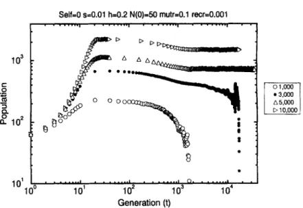
4.3. Sexual reproduction

Fig. 10 shows the results obtained for outcrossing populations Self=O with recombination rate recr = 0.001 for a initial population o f N ( 0 ) = 50 individuals and different environmental carrying capacities. In contrast with the results shown in Fig. 6, here the action o f recombination represents a strong mechanism to avoid extinction. For N,,ox = 1000 and 3000 we observe the same path to extinction as described to the selfing population. For Nmax = 5000 the population seems to stabilize around 700 individuals after 35 000 generations, though an extremely slow decay can be observed in the population mean fitness (discussed below). Finally, for Nm~x = 10 000 the population seems to stabilize around 1500 individuals. In comparison with the results obtained for asexual populations, here the extinction was avoided for a much smaller population. For asexual populations the stabilization was observed only for a population o f about 100 000 individuals (Fig. 6) whilst here this is observed for 700 individuals. However, even this small sexual population which survived is an order o f magnitude greater than that supposed, for instance, by Charlesworth et al. [16].

(15)

1.00

¢R ¢0

._=

0.90

LL

0.80

0o

i

D ~ [3~p

Self=0 s=0.01 h=0.2 N(0)=50 mutr=0.1 recr=0.001

= g w

O

o%~.

AO

I I I ~ I •

101 102 103 104

Generation (t)

.. .. ... . ! •

0.905

0.895 03 104

0.91

0"90103

10 4

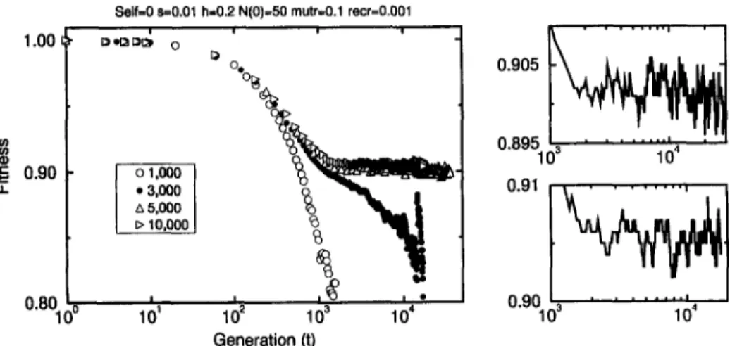
Fig. 11. Time evolution of the population mean fitness for the simulations showed in Fig. 10. The upper fight plot shows a detail of the fitness obtained for N,n~ = 5000, where a slow decreasing trend seems to appear in the last 20000 generations. The lower fight plot shows a detail for N , nax = 10000, where an opposite trend seems to appear in the last 10000 generations.

in the fitness, though there are fluctuations which do not allow a conclusive statement. However, for Nmax = 10000 an opposite trend might be assumed. There, a very slight increase in the fitness seems to appear after 10000 generations, though a simulation for just one sample for longer periods (40 000 generations) does not show a conclusive result. It is important to emphasize that in this model only forward mutations are accepted and the recombination process seems to produce better genotypes. This fact might confirm that traditional Muller's picture (cited in Ref. [5]) on the higher probability of getting better genomes in sexually reproductive populations than in asexually ones.

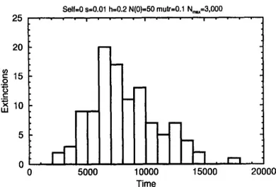
Recently, Biirger and Lynch [19] have observed that, even with the knowledge of the mean time to extinction for a given set of parameters describing the evolution of a species (or a population), it is not possible to draw conclusions about the evolution of a single population. The stochasticity of the extinction process can be observed in Fig. 12. There, a histogram of frequency of extinctions versus time to extinction is shown. It represents the results obtained for the case Nmax = 3000 discussed in Fig. 10. The mean time to extinction is ?e = 8185 generations (averaged over 110 samples), whereas the maximum and minimum observed times are t m~x = 17 120 and t~ i" = 2500 generations. It is remarkable that the same kind of stochastic process can be observed also in the Penna model for biological ageing, when the mutations events are Poisson distributed [23].

5. C o n c l u s i o n s

(16)

20

A.T. Bernardes/ Physica A 230 (1996) 156-173

Self=0 s=0.01 h=0.2 N(0)=50 mutt=0.1 N,~=3,000

171

= 1 5

.fl

,,'5, lO

0 5000 25

10000 15000 20000 Time

Fig. 12. Frequency of extinctions versus time to extinction obtained for the simulations showed in Fig. 10 for N, nax = 3000. This result was obtained for 110 statistically independent runs.

in the population mean fitness in evolutionary populations. Traditionally, the dynamical aspect of evolution was ignored by assuming that the population should attain an equilibrium state. However, it seems that nature prefers to work out of equilibrium in several contexts and it might be assumed the same for the evolution of the populations, since life is clearly a nonequilibrium phenomenon. Different types of attractors can be found when modeling evolutionary systems: oscillatory pattems (like in the Lotka-Volterra equations), self-organized criticality in extinction events, a fixed point (extinctions being the example we have discussed here), etc. [29]. Hence, the fixed population equilibrium must be understood as a very artificial state or a metastable state where a population stays for a given period (how long it is not possible to state in advance) [12, 19].

Firstly, we have discussed the equilibrium assumption and showed that signs of a nonequilibrium dynamics can be observed in earlier computer simulations. The problems in nonequilibrium dynamics are very hard to treat analytically and there has been an increased use of computer simulations. Working in a model introduced by Charlesworth et al. we observed three different aspects when performing the simulations by using the fixed population prescription:

- the population mean fitness shows a scaling behaviour which is different under weak or strong selection, but for a fixed population the fitness always decays with time; - under strong selection, the existence of recombination produces a higher fitness, but

better results appeared for selfing populations. Under weak selection, the existence of recombination had little effect for selfing populations, though for outcrossing populations a slight increase in the fitness was obtained with recombination;

(17)

These different aspects show how the use of the fixed population prescription ob- scures the evolution of the populations and we have adopted a time-changing population, by introducing a fixed reproductive rate and an environmental carrying capacity. In order to describe the path to extinction in this new scenario, we have just taken into account variations in the selection coefficient s and in the environmental carrying capacity Nm~x for different reproductive regimes: selfing populations without recombination (asexual) and outcrossing with recombinations (sexual).

Our results confirm the assumption that under strong selection harmful mutations are unlikely to be fixed in the population. However, as discussed by Kondrashov [20], the existence of very slightly deleterious mutation might lead to a high mutation load if a long period is taken into account. Thus, we focused our attention here in the region of weak selection.

For asexual population, we observed the extinction of populations which reached a maximum size of about 20 000 individuals. The value of the fitness in this case is very different from that which would be calculated by using the traditional expressions. The variation of the fitness with the selection coefficient is again nonmonotonic. It is important to say that our results are in good agreement with that obtained by Gabriel et al. [27] in a different model.

Moreover, the stochasticity of extinction events was observed. It shows that is very difficult to state in advance the temporal behaviour of a single population, as recently pointed out by Biirger and Lynch [19].

However, the most important aspect observed is the difference in the evolution when populations without and with recombination are compared (see Figs. 6 and 10). The powerful mechanism of recombination can be observed when simulating a sexual population. Populations of about 1000 individuals escaped from extinction and for larger populations, a slight trend to increase the mean fitness was noticed, though our re- suits are not yet conclusive. Our results confirm the basic assumptions of the evolution of sex [30] and also confirm those obtained through Monte Carlo simulations in the Penna model [23]. They disagree with those obtained by Redfield [31], who obtained better results for asexual reproduction. Thus, our results might suggest an answer to the question addressed by Kondrashov [20]: Why have we not died 100 times over? Even considering the supposed costs of recombination [30] or still the assumption of a higher male mutation rate [32], it is well known that all the living beings either can produce genetically diverse offspring (by recombination) or, at least, are capable to mimic the recombination process. Our results showed that recombination strongly reduces the probability of extinction.

(18)

A.T. Bernardes/Physica A 230 (1996) 156-173 173

Acknowledgements

I thank B. Charlesworth and A. Kondrashov for addressing me some important ques- tions during the development of this work, D. Stauffer for many suggestions and helpful discussions. This work is partially supported by the Brazilian Agency Conselho Na- cional para o Desenvolvimento Cientifico e Tecnol6gico - CNPq. Computer simulations were performed on several sun workstations, DEC-Alpha and Silicon Graphics stations at RRZ, Cologne University, and Intel Paragon at KFA Jiilich.

References

[1] J.B.S. Haldane, Amer. Naturalist 71 (1937) 337. [2] S. Wright, Genetics 16 (1931) 97.

[3] J.F. Crow, Human Biol. 30 (1958) 1.

[4] M. Kimura, T. Maruyama and J.F. Crow, Genetics 48 (1963) 1303. [5] J.F. Crow and M. Kimura, Amer. Naturalist 99 (1965) 439.

[6] J.F. Crow and M. Kimura, An Introduction to Population Genetics Theory (Harper and Row, New York, 1970).

[7] H.J. Muller, Mutation Res. 1 (1964) 2. [8] J. Felsenstein, Genetics 78 (1974) 737.

[9] R. Heller and J.M. Smith, Genetical Res. (Cambridge) 32 (1979) 289. [10] A. Kondrashov, Genetics 111 (1985) 635.

[11] P. Pamilo, M. Nei and W.-H. Li, Genetical Res. (Cambridge) 49 (1987) 135. [12] M. Lynch and W. Gabriel, Evolution 44 (1990) 1725.

[13] A. Kondrashov, Nature 336 (1988) 435.

[14] D. Charlesworth, M.T. Morgan and B. Charlesworth, Genetical Res. (Cambridge) 59 (1992) 49. [15] D. Charlesworth, M.T. Morgan and B. Charlesworth, J. Heredity 84 (1993) 321.

[16] D. Charlesworth, M.T. Morgan and B. Charlesworth, Genetical Res. (Cambridge) 61 (1993) 39. [17] M. Lynch, R. B/irger, D. Butcher and W. Gabriel, Journal of Heredity 84 (1993) 339. [18] A. Kondrashov, Genetics 136 (1994) 1469.

[19] R. Biirger and M. Lynch, Evolution 49 (1995) 151. [20] A. Kondrashov, J. Theor. Biol. 175 (1995) 583.

[21] G.C. Williams, Evolution 11 (1957) 398; M.R. Rose, Evolutionary Biology of Aging (Oxford Univ. Press, New York, 1991 ); L. Partridge and N.H. Barton, Nature 362 (1993) 305; D. Houle et al., Genetics 138 (1994) 773; B. Charlesworth, Evolution in Age-Structured Populations, 2nd Ed. (Cambridge Univ. Press, Cambridge, 1994).

[22] T.J.P. Penna, J. Stat. Phys. 78 (1995) 1629; T.J.P. Penna and D. Stauffer, Int. J. Mod. Phys. C 6 (1995) 233; A.T. Bernardes and D. Stauffer, Int. J. Mod. Phys. C (1996), in press.

[23] A.T. Bernardes, in: Annual Reviews of Computational Physics, Vol. IV, ed. D. Stauffer (World Scientific, Singapore, 1996), in press.

[24] A.T. Bernardes, J. Phys. I France 5 (1995) 1501.

[25] S. Vollmar and S. Dasgupta, J. Phys. I France 4 (1994) 817. [26] J. Thorns, P. Donahue and N. Jan, J. Phys. 1 France 5 (1995) 935. [27] W. Gabriel, M. Lynch and R. B/irger, Evolution 47 (1993) 1744.

[28] S. Moss de Oliveira, T.J.P. Penna and D. Stauffer, Physica A 215 (1995) 298; H. Puhl, D. Stauffer and S. Roux (1995) Physica A 221 (1995) 445; S. Feingold, Physica A (1996), in press.

[29] G.D. Ruxton, J. Theor. Biol. 175 (1995) 595; P. Bak and K. Sneppen, Phys. Rev. Lett. 71 (1993) 4083; P. Sibani, M.R. Schmidt and P. Alstrom, Phys. Rev. Lett. 75 (1995) 2055; for a review and evolutionary models see N. Vandewalle and M. Ausloos, in Annual Reviews of Computational Physics, Vol. llI, ed. D. Stauffer (World Scientific, Singapore, 1995) pp. 45-86,