A dynamical multibody approach for guitar modelling
incorporating string geometric nonlinear effects
V. Debut1,2, J. Antunes1,2
1
Instituto de Etnomusicologia - Centro de Estudos em Música e Dança, Faculdade de Ciências Sociais e Humanas, Universidade Nova de Lisboa, Avenida de Berna, 26C, 1069-061 Lisbon, Portugal. [email protected] 2
Centro de Ciências e Tecnologias Nucleares, Instituto Superior Técnico, Universidade de Lisboa, Estrada Nacional 10, Km 139.7, 2695-066 Bobadela LRS, Portugal. [email protected]
Most musical instruments consist on dynamical subsystems connected at a number of constraining locations. For physical sound synthesis, one important difficulty deals with the manner to enforce these coupling constraints. While standard techniques include the use of Lagrange multipliers or penalty methods, we explore in this paper a different approach, the Udwadia-Kalaba (U-K) formulation, which is rooted on analytical dynamics but avoids the use of Lagrange multipliers. Following our recent work, we generalize this modelling framework to a multibody flexible system such that each component is defined by its unconstrained modal basis, and then compute the string/body coupled dynamics of a guitar. Moreover, the generality of this computational technique is demonstrated by incorporating the string geometrical nonlinear effects in the model, using the Kirchoff-Carrier (K-C) simplified approach. The guitar model obtained is computationally effective and the illustrative results presented highlight the significance of the nonlinear string effects for plucked string instruments, which lead to clearly audible modal coupling terms and frequency gliding effects.
1. Introduction
Most musical instruments consist on a set of dynamical subsystems connected at a number of constraining locations, through which the vibratory energy flows or tuning can be achieved. Coupling is therefore an essential feature in instrument modelling and, when addressing physically-based synthesis, most modelling and computational difficulties are connected with the manner in which the coupling constraints are enforced. Typically, these are modelled using standard techniques such as Lagrange multipliers or penalty methods, each one with specific merits and drawbacks. In this paper we explore a different approach, the Udwadia-Kalaba (U-K) formulation, originally proposed in the early 90s for discrete constrained systems [1], which is anchored on analytical dynamics but avoids the use of Lagrange multipliers.
Up to now, this general, very elegant and appealing formulation has been nearly exclusively used to address conceptual systems of discrete masses or articulated rigid bodies, namely in robotics. To the authors best knowledge, the single exception in the literature is the work by Pennestri et al. [2], who addressed a flexible slider-crank mechanism modelled using a Finite Element Timoshenko beam formulation. However, in spite of the possible natural extension of the U-K formulation to deal with flexible systems modelled through their unconstrained modes, such promising approach is surprisingly absent from the literature.
In our recent work we developed the potential of combining the U-K formulation for constrained systems with the modal description of flexible structures, in order to achieve reliable and efficient computations of the dynamical responses. This modelling approach was shown to be particularly effective, in particular for simulating the transient responses of musical instruments, as demonstrated by computing the dynamical responses of a guitar string coupled to the instrument body at the bridge [3].
2. Theoretical formulation
2.1. Basic U-K formulation
Following on from Gauss' Principle of Least Action, Udwadia & Kalaba developed an elegant analytical treatment for the dynamics of discrete mechanical systems subjected to constraints [1]. In general mathematical terms, they proposed the following standard form for the study of the constrained dynamics:
e c
Mx
F
F
(1)which expresses the system vector response
x
( )
t
as the result of the application of an applied force fieldF
e( )
t
and some additional forces
F
c( )
t
stemming from a set of constraints. In the same manner as other multibody formulations, the U-K approach uses an alternative expression of the usual constraint equationsΨ
p( , , )
x x
t
0
(p
1, 2,
,
P
), obtained by differentiation with respect to time, which leads to a set of linear equality relations in terms of the system accelerations, as:( , , )
t
( , , )
t
A x x
x
b x x
(2)where
A x x
( , , )
t
is referred to as the constraint matrix andb x x
( , , )
t
is a known vector. Their main result isthen to provide an explicit expression for the constrained dynamical response
x
( )
t
and the constraint force vectorF
c( )
t
, which are respectively given by the fundamental equations:
1/ 2
u u
x
x
M
B
b
Ax
(3)
1/ 2
c u
F
M B
b
Ax
(4)where
B
( )
t
A
( )
t
M
1/ 2 andB
stands for the Moore-Penrose pseudo-inverse of matrixB
. Vector
x
u( )
t
represents the dynamical response of the system when no constraint is imposed, which is computed as:1
u e
x
M F
(5)while the second term in the right-side hand of (3) accounts for the influence of the constraints on the system dynamics. The superlative elegance of the U-K formulation lays in the fact that it encapsulates, in a single explicit equation, both the dynamical equations of the system and the constraints applied. It allows, if needed, the computation of the constraining forces through (4). No additional variables, such as Lagrange multipliers, are needed. Equations (3)-(5), which may be applied to linear or nonlinear, conservative or dissipative systems, can be efficiently solved using a suitable time-step integration scheme for any given excitation. It can be noticed that, if no constraints are applied, the constraint force vector - and thus the correcting term in (3) and (4) - is nil, so that the unconstrained results are recovered.
2.2. Modal U-K formulation
Although originally proposed for constrained discrete systems, the Udwadia-Kalaba formulation can be extended to deal with continuous flexible systems constrained at some specific points. Let us consider a modal framework in which any physical quantity
x r
( , )
t
varying in space and time is expressed as a modal superposition:1
( , )
( )
( )
N
n n
n
t
φ
q t
x r
r
x
Φ
q
(6)where vector
q
( )
t
contains the modal amplitudesq t
n( )
, while the columns of matrixΦ
are the modeshapes( )
n
φ
r
appropriate to the boundary conditions. Then, a formulation very similar to the previous U-K equation (3) can be derived for the modal responses of the constrained system. Projecting as usual the dynamical equations on the modeshapes of the system, this yields:
1/ 2
u u
b
where
q
u are the modal accelerations of the unconstrained system,T
M
M
are the modal masses,( )
t
A
( )
t
cA
are the modal constraint equations (with the modal matrix
c defined at the constraintlocations) and
B
( )
t
A
( )
t
M
1/ 2. The modal constraining forces may be deduced as:
1/ 2
c u
b
F
M
B
Aq
(8)Finally, from the knowledge of the constrained modal responses, the physical responses are obtained using (6), while the physical constraining forces can be computed from (8) as:
(
)
T
c c c
F
F
(9)2.3. Dynamically coupled subsystems
The application of the U-K modal formulation to a multibody set of
S
vibrating subsystems, coupled through a number of kinematic constraints, can now be considered. Using a modal description, the unconstrained dynamics of each subsystem subjected to an external force field can be classically written as a set of modal equations:(
,
)
,
1, 2,
,
s s s s s s s s s s
nl ext
s
S
M q
C q
K q
F
q q
F
(10)where, for each subsystem
s
,M
s,C
s andK
s are diagonal matrices of modal parameters, while s( )
ext
t
F
and(
,
)
s s s
nl
F
q q
are the modal force vectors stemming from the external and nonlinear force fields, which are obtained by projection of the physical forces on the modal basis. According to (7), the U-K approach requires the computation of the modal accelerations of the unconstrained system, which are simply given by:1
(
)
,
1, 2,
,
s s s
u
s
S
q
M
F
(11)where
F
s denotes the vector of all the constraint-independent modal forces:(
,
)
,
1, 2,
,
s s s s s s s s s
ext nl
s
S
F
F
C q
K q
F
q q
(12)for which it is assumed that the vectors of modal constrained displacements and velocities are known at each time-step. Assembling the modal quantities of the
S
subsystems in compact vectors and block matrices, theunconstrained modal accelerations of the coupled system u
1u,
u2,
,
uS
T
Q
q q
q
read:
1
( , )
u ext nl
Q
M F
C
Q
K
Q
F
Q Q
(13)where
Q
q q
1,
2,
,
q
S
Tand 1 2,
,
,
S T
Q
q q
q
denote the constrained modal displacements and velocities, whileM
,C
andK
are block diagonal matrices set up by the submatrices of the modal parameters of the various subsystems, built according to:1 1 1
2 2 2
;
;
S S S
0
0
0
0
0
0
0
0
0
0
0
0
0
0
0
0
0
0
M
C
K
M
C
K
M
C
K
M
C
K
(14)with the modal parameters in the diagonal matrices
M
s,C
s andK
s given respectively as:2 2
( )
( )
;
2
;
(
)
s
s s s s s s s s s s s s
n n n n n n n n n
D
where
ρ
( )
r
s is the mass density,ω
ns are the modal circular frequencies,ζ
ns are the modal damping ratios and( )
s s
n
φ
r
are the modeshapes of each subsystem. The modal forcesF
ext( )
t
and nl( , )
Q Q
F
are computed byprojecting the corresponding force fields
f
ext andf
nl on the subsystems modeshapes:f ( , ) f ( , )
( )
,
1, 2,
,
s
s s s s s s
n ext nl n s
D
F
r
t
r
t
φ
r
d
r
n
N
(16)Besides the unconstrained equation (13), the second set of equations to be considered in the U-K formulation concerns the
P
constraints which couple the various subsystems, defined at specific locationsr
cs. In most practical situations, these are amenable to the standard form:( , , )
t
b
( , , )
t
A Q Q
Q
Q Q
(17)where
A
( )
t
A
( )
t
c with:1
2
c c c
S c
0
0
0
0
0
0
Φ
Φ
Φ
Φ
(18)
where the
Φ
cs contain the modeshape vectors of each subsystem at the constraint locationsr
cs. Finally, from:
1/ 2
u u
b
Q
Q
M
B
AQ
(19)one can compute at each time-step the constrained modal accelerations.
3. String geometric nonlinearity
3.1. The Kirchoff-Carrier formulation
For a vibrating string, inclusion of the geometric nonlinear terms leads to coupling of the three motion directions, axial
X t
( )
and transverseY t
( )
andZ t
( )
:
2 2
0
2 2
2 2 2
2 2
0
2 2
2 2
0
2 2
1
with
1
X
X
X
x
S
ES
T
ES
t
x
x
R x
Y
Y
Y x
R
X
Y
Z
S
ES
T
ES
t
x
x
R x
x
x
x
x
Z
Z
Z x
S
ES
T
ES
t
x
x
R x
ρ
ρ
ρ
(20)
However, this general formulation is numerically awkward, hence a number of simplified formulations are used in practice, often based on Taylor series developments from (20). Here the simple nonlinear Kirchoff-Carrier formulation has been implemented, which deals with the axial string motions in a quasi-static manner, thus being adequate for modelling the nonlinear behaviour of the lower-frequency string modes. The quasi-static hypothesis on
X t
( )
enables suppressing the axial motion from formulation (20) which, after some developments, leads to the following form for the transverse motions:2 2 2 2
0 0
2 dyn
( )
2;
2 dyn( )
2Y
Y
Z
Z
S
T
T
t
S
T
T
t
t
x
t
x
ρ
ρ
(21)2 2
0
( , )
( , )
( )
2
dyn
L
ES
Y x t
Z x t
t
dx
L
x
x
T
(22)
Then, through equations (21)-(22), the two transverse motions are coupled, the geometric nonlinearity being overall of the cubic type.
3.2. Nonlinear K-C modal terms
In the framework of the present modal model, for any given string equations (21)-(22) are projected on the unconstrained string modal basis, using equations (16), with the string displacements expressed in terms of the string modal responses, equation (6). After performing the space integrations, the following nonlinear modal forces are obtained:
2 2
2 2
( )
( )
( ) ;
( )
( )
( )
2
2
Y Y Z Z
n n dyn n n dyn
F
t
n q t T
t
F
t
n q t T
t
L
L
π
π
(23)with the dynamical string tension:
2
2 2
2 2
2
1 1
( )
( )
( )
4
Y Z
Y Z
dyn m m
N N
m m
ES
T
t
m
q t
m
q t
L
π
(24)
Results (23)-(24) clearly show the quadratic nature of the motion-dependent nonlinear tension, as well as the cubic modal coupling due to the geometric nonlinearity.
4. Guitar model
4.1. Unconstrained modal equations
For illustrative purpose, we formally address the coupled dynamics of a guitar string and body, coupled at the instrument bridge, and including the influence of a stopping finger along the fingerboard to control the frequency of the plucked tone. The vibrating elements are modelled using the modal U-K formulation, using the unconstrained modal basis of the string and of the instrument body, while the string/finger coupling is thought as a simple physical constraint acting on the vibratory motion of the string.
According to (10), the forced response of the string can be formulated as a set of NS modal ODEs and,
similarly, as a set of NB modal ODEs is formulated for the body. Then, ignoring for the moment the string/body
coupling constraint at the bridge and the string motion constraint at the musician’s tuning finger, the matrix equation (13) which expresses the unconstrained modal dynamics of the excited nonlinear string, as well as the modal dynamics of the body, reads:
1
1
(
)
(
)
(
)
S S S S S S S S S
u exc nl
B B B B B B
u
0
0
0
0
0
0
0
0
q
M
F
C
q
K
q
F
q
q
M
C
q
K
q
(25)where vector
F
excS( )
t
is the set of modal string forces corresponding to the pluck excitation. Here, for simplicity, only a single motion direction of the string (normal to the instrument soundboard) is addressed, however the other direction might be easily included as well. The modal force terms of the vectorF
nlS(
q
S)
, stemming from the string geometric nonlinearity, are obtained from (23)-(24):2 2 2 4
2 2
2 2 2 2 2
2 3
1 1
( )
( )
( )
( )
( )
( )
( )
2
2
4
8
S S
S S S S S S
n n dyn n m n m
N N
m m
ES
ES
F t
n q t T
t
n q t
m q t
n q t
m q t
L
L
L
L
π
π
π
π
The modal matrices in (25) are block diagonal. Then, for linear subsystems, the unconstrained dynamics would behave as if the modal amplitudes were independent. However, the modal coupling due to the string nonlinearity leads to coupled modal equations, even for the unconstrained dynamics, see (26).
4.2. Modal constraint equations
String/body constraint
Assuming a rigid transmission at the bridge between the string and the body, the modal equations of the constrained system are required to satisfy a set of constraint modal equations, stemming from the condition that, at the bridge location, the string motion
Y
S(
x t
B, )
must be the same as the instrument body motion at the stringlocation
Y
B( , )
r
St
. Formally, this results in the condition:
,
,
0
(
)
T( )
( )
T( )
0
S B S S B B
B S c B c S
Y
x t
Y
r
t
x
q
t
r
q
t
(27) with the modeshape vectors:1 2 1 2
(
)
(
)
(
)
(
)
;
( )
( )
( )
( )
S B
T T
S S S S B B B B
c
x
B
φ
x
Bφ
x
Bφ
Nx
B
c S
φ
Sφ
Sφ
N S
r
r
r
r
(28)String/finger constraint
Following a simple strategy for modelling the influence of the string/finger interaction, the string motion
(
, )
S f
Y
x t
must be nil at the finger locationx
F. To refine the modelling and account for the finite width of thefinger, several rigid constraint can be thought at close locations
i f
x
(withi
1, 2,...,
F
), so that a set ofF
string/finger constraint equations is obtained:
( ),
0
( )
( )
0
,
1, 2,...,
i i
T
S S S
f f
Y
x
t t
t
q
t
i
F
(29) with the modeshape vectors:1 2
(
)
(
)
(
)
(
)
,
1, 2,...,
i i i S i
T
S S S S
c
x
f
φ
x
fφ
x
fφ
Nx
f
i
F
(30)Finally, assembling the various constraint conditions (27) and (29) into compact form, the global constraint equation (17) reads:
1
(
)
( )
0
0
( )
( )
( )
0
( )
F
T T
S B
c B c S
T
S S
f
B
T S
f
x
t
t
t
t
r
0
0
q
q
(31)4.3. Time-domain solution
For the case of interest, the constrained modal accelerations are readily computed from (19), by formulating the efficient recurrence:
1/2 1/2
with
S S S
S S
u u u
B B B
B B
u u u
1
q
q
q
q
q
B A
W
W
B A
q
q
q
q
M
q
M
(32)5. Illustrative computations
5.1. System parameters
The present computations pertain to a single string with parameter values experimentally identified [5] coupled to a guitar body whose modes were experimentally identified in [3]. The computed string (
A
2) is tuned to afundamental of f1110 Hz, with length (from nut to bridge) L0.65 m, axial tensioning force T0 73.9 N, mass per unit length 3
3.6110 kg/m S
ρ
, transverse wave propagation velocity
c
t
T/ρS 143 m/s andinharmonicity parameter (bending stiffness of a non-ideal string) 5 2
4 10 Nm
BEI . Also, we have
experimentally identified for this string the value ES3.73 10 N3 . Then, for the unconstrained string used in our dynamical computations (pinned at the nut and "free" at the bridge), the inharmonic modal frequencies and unconstrained modeshapes are computed for 150 modes (up to 20 kHz) as:
2
(2
1)
1
;
( )
sin
with
2
2
2
S t S
n n n n n n
c
B
n
f
p
p
x
p x
p
T
L
π
φ
π
(33)and the modal masses are obtained as
m
nS
0.5
ρ
S L
/
(
n
)
. Concerning the string modal damping, complexdissipative phenomena must be accounted for, as discussed in [6], where the following pragmatic formulation for modal damping was adopted:
20
2
(2 ) 1
2
S
F A n B n
n
S n
T f Bp
T Bp
η η π η
ζ
(34)
Here the loss coefficients, loosely described as "internal friction", "air viscous damping" and "bending damping", were fitted from experimental data and are for this string
η
F
7 10
5,η
A 0.9 andη
B
2.5 10
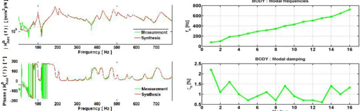
2. As should be expected, none of the unconstrained string modes of this modal basis approaches the fundamental frequency 110 Hz of the pinned-pinned string. However, when these modes are coupled by the string/body constraint at the bridge, the fundamental frequency will be recovered, as it should. Figure 1 illustrates the experimental transfer function of the guitar body, at the bridge, as well as the corresponding modal parameters identified in the frequency range 0~800 Hz, see [3].Figure 1:Instrument body: Transfer function at the bridge (left); Modal frequencies and damping values (right).
5.2. Illustrative computational results
In the simulations presented, we computed the string responses for a tuning string constraint on the fingerboard at
x
F 0.33L, using a linear force ramp 0-10 N during the initial 0.01 sec of the simulation, for the string excitation applied near the bridge atx
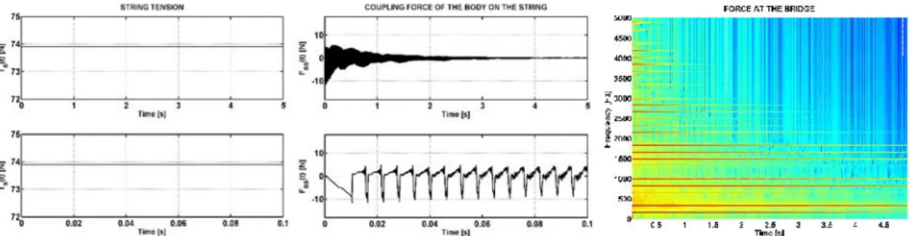
E 0.90L. Simulated time is 5 sec using an integration time-step of105Figure 2:Linear string simulation: Variable tension (left); String/body force (center); Spectrogram (right).
Figure 3:Nonlinear string simulation: Variable tension (left); String/body force (center); Spectrogram (right).
6. Conclusions
In this paper we developed a new approach for computing the dynamics of coupled flexible systems, based on the general formulation of Udwadia-Kalaba, which is becoming increasingly popular in the field of multibody dynamics. The general U-K equations were adapted to address coupled subsystems, defined in terms of their unconstrained modal basis. This approach shows a considerable potential to deal effectively with the dynamics of physically modelled musical instruments, and the formulation developed was applied for modelling a guitar, including the fully coupled dynamics of a string, tuned on the fingerboard, and the instrument body. String geometric nonlinearity was addressed through a modal implementation of the Kirchoff-Carrier model. The significance of the various modelled effects was highlighted in the illustrative computations presented.
7. Acknowledgements
The authors acknowledge the Fundação para a Ciência e a Tecnologia for the financial support of INET-md and C2TN through the UID/EAT/00472/2013 and UID/Multi/04349/2013 projects.
8. References
[1] F.E. Udwadia, R.E. Kalaba. A new perspective on constrained motion. Proceedings of the Royal Society, A439, (1992), 407-410.
[2] E. Pennestri, P.P. Valentini, D. de Falco. An application of the Udwadia-Kalaba dynamic formulation to flexible multibody systems. Journal of the Franklin Institute, 347, (2010), 173-194.
[3] J. Antunes, V. Debut. Dynamical computation of constrained flexible systems using a modal Udwadia-Kalaba formulation: Application to guitar modelling. International Symposium on Musical and Room Acoustics (ISMRA 2016), La Plata, Argentina, 11-13 September 2016.
[4] M. Marques, J. Antunes, V. Debut. Coupled modes and time-domain simulations of a twelve-string guitar with a movable bridge. Stockholm Music Acoustics Conference (SMAC 2013), Stockholm, Sweden, 30 July-3 August 2013.
[5] V. Debut, J. Antunes, M. Marques, M. Carvalho. Physics-based modeling techniques of a twelve-string Portuguese guitar: A non-linear time-domain computational approach for the multiple strings/bridge/soundboard coupled dynamics. Applied acoustics, 108, (2016), 3-18.