BCG - Boletim de Ciências Geodésicas - On-Line version, ISSN 1982-2170 http://dx.doi.org/10.1590/S1982-21702014000100012
THE COMPUTATION OF THE GEOID MODEL IN THE
STATE OF SÃO PAULO USING TWO METHODOLOGIES
AND GOCE MODELS
O cálculo do modelo geoidal no estado de São Paulo utilizando duas metodologias e os modelos do GOCE
GABRIEL DO NASCIMENTO GUIMARÃES1 DENIZAR BLITZKOW2
RICCARDO BARZAGHI3
ANA CRISTINA OLIVEIRA CANCORO DE MATOS2
1Instituto de Geografia da Universidade Federal de Uberlândia
Engenharia de Agrimensura e Cartográfica 2Escola Politécnica da Universidade de São Paulo - EPUSP
LTG - Laboratório de Topografia e Geodésia 3Politecnico di Milano – POLIMI
DIIAR – Sezione Rilevamento
[email protected]; [email protected]; [email protected]; [email protected]
ABSTRACT
The purpose of this manuscript is to compute and to evaluate the geoid model in the State of São Paulo from two methodologies (Stokes’ integral through the Fast Fourier Transform - FFT and Least Squares Collocation – LSC). Another objective of this study is to verify the potentiality of GOCE-based. A special attention is given to GOCE mission. The theory related to Stokes’ integral and Least Squares Collocation is also discussed in this work. The spectral decomposition was employed in the geoid models computation and the long wavelength component was represented by EGM2008 up to degree and order 150 and 360 and GOCE-based models up to 150. The models were compared in terms of geoid height residual and absolute and relative comparisons from GPS/leveling and the results show consistency between them. In addition, a comparison in the mountain regions was carried out to verify the methodologies behavior in this area; the results showed that LSC is less consistent than FFT.
The computation of the geoid model in the State of... 1 8 4
RESUMO
O objetivo deste artigo é calcular e avaliar o modelo geoidal no Estado de São Paulo a partir de duas metodologias (a integral de Stokes por meio da Transformada Rápida de Fourier – FFT e a Colocação por Mínimos Quadrados – LSC). Outro objetivo deste estudo é verificar a potencialidade dos modelos baseados no satélite GOCE. Uma atenção especial é dada à missão GOCE. A teoria relacionada à integral de Stokes e a LSC também é discutida nesse trabalho. A decomposição espectral foi empregada no cálculo dos modelos geoidais e os longos comprimentos de onda foram representados pelo EGM2008 até grau e ordem 150 e 360 e pelos modelos do GOCE até 150.Os modelos foram comparados em termos de resíduo da altura geoidal e de comparações absolutas e relativas a partir de pontos GPS sobre nivelamento, sendo que os resultados mostram consistência entre si. O modelo geoidal no Estado de São Paulo tem uma consistência de 0,20 m em relação aos pontos GPS sobre nivelamento. Uma comparação na região montanhosa também foi realizada para verificar o comportamento das metodologias naquela região; os resultados mostraram que a LSC é menos consistente do que a FFT.
Palavras-chave: Geodésia; Modelo Geoidal; GOCE; Gravidade.
1. INTRODUCTION
Geodesy is concerned with the Earth’s orientation parameters in the space, the shape and dimension of the Earth and estimation of its external gravity field. The shape computation of the Earth is carried out by the knowledge of the gravity field involving the mass distribution and the rotational effect of the planet. The determination of the potential function of the referred field should involve what is called “Geodetic Boundary-Value Problem”.
Guimarães, G. N. et al. 1 8 5 equipments: GPS (Global Satellite System), DORIS (Doppler Orbit determination and Radio positioning Integrated on Satellite) and laser system. In this paper, GOCE-based models will be used, beyond EGM2008.
Once the geoid model is computed, the most common way to analyze its quality is comparing over GPS observations on Bench Marks of spirit leveling network. The geoid height obtained from ellipsoidal height (GPS) minus normal height (spirit leveling) allows comparing with the geoid model height. Moreover, the comparison with recent GGMs is another option. In this case it is also possible to verify the quality of the geopotential model and the compatibility between them. The comparison involving two different methodologies can be done to ensure if they have the same behavior and to provide information of their consistency.
2. THE GOCE MISSION
The spatial era contributed to the GGMs. The first model was published in the 1960s. The 1990s initialized the so called gravity decade. The modern gravitational missions were developed with specific objectives. From these missions three satellites were projected: CHAMP (CHAlleging Minisatellite Payload) (REIGBER et al., 1996), GRACE (Gravity Recovery And Climate Experiment) (GRACE, 1998) and GOCE (Gravity field and steady-state Ocean Circulation Explorer) (ESA, 2006). The last one was developed by the European Space Agency (ESA) and the main objective of the mission is to obtain a gravitational field model at the ~ 1-2 cm accuracy level for geoid height and at the 1-2 mGal level for gravity anomalies, and to achieve these results at a spatial resolution better than 100 km. Since then, several geopotential models of different degree and order have been published.
Rapp (1998) reviewed the past and future developments in geopotential modeling. A GGM consists of a set of numerical values for certain parameters, the statistics of the errors associated with these values (as expressed in their error covariance matrix), and a collection of mathematical expressions and algorithms that allow a user to perform synthesis and error propagation (see Pavlis, 2010 for more details).
The GOCE satellite was developed by the European Space Agency and deployed a gravity gradiometry in space to produce homogeneous, highly accurate, near-global maps of the Earth’s static gravitational field (e.g. Visser et al., 2001; Drinkwater et al., 2007). According to the mentioned requirements, the GOCE mission can represent the gravitational potential by spherical harmonic functions completed at least to degree and order 200, but 250 is envisaged.
The computation of the geoid model in the State of... 1 8 6
Table 1 – Data periods of solutions and releases.
Solution From d/m/y To d/m/y Number of days
DIR_R4 01/11/2009 01/08/2012 1004 DIR_R3 01/11/2009 19/04/2011 536 DIR_R2 01/11/2009 30/06/2010 242 DIR_R1 01/11/2009 11/01/2010 72 TIM_R4 01/11/2009 19/06/2012 962 TIM_R3 01/11/2009 17/04/2011 534 TIM_R2 01/11/2009 05/07/2010 247 TIM_R1 01/11/2009 11/01/2010 72 SPW_R2 30/10/2009 05/07/2010 248 SPW_R1 30/10/2009 11/01/2010 74
3. GEOID ESTIMATION
The Boundary-Value Problem consists in the determination of the gravity field external to the masses where the boundary surface is unknown. Stokes proposed a formulation to obtain the disturbing potential as a function of the gravity anomaly on the geoidal surface. However, this proposition implies in some difficulties because it is a problem internal do the masses. A new formulation was proposed by Molodensky. It is a problem external to the masses, which uses the physical surface as the boundary. In this sense, there is no need for the knowledge, even approximately, of a density distribution model within the crust between the geoidal and the physical surface. However, this surface has no physical meaning as the geoidal surface, because it is not an equipotential surface. The expression proposed by Molodensky is a nonlinear integral that cannot be solved directly. The solution is to linearize by introducing suitable approximate values. In this case, the real Earth is substituted by the normal Earth and the approximate solution for the boundary surface is the telluroid. What is computed is not the geoid, but the quasi-geoid. Gravity anomaly and vertical deflections are referred to the physical surface and not to the geoidal surface. Moreover, geoid heights are substituted by height anomalies and orthometric heights are replaced by normal heights. In this paper the terminology geoid and geoid height will be used instead quasi-geoid and height anomaly.
3.1 Stokes’ Integral
Guimarães, G. N. et al. 1 8 7 the geoid. This reduction leads to a mass redistribution, which means the creation of a fictitious Earth with a gravity potential changed. The geoid height obtained by Stokes’ integral is represented by the separation between the reference ellipsoid and a "fictitious geoid", called geoid. The difference between the geoid and the co-geoid it is called indirect effect.
The modified Stokes’ integral expression to obtain the geoid height in this manuscript (ELLMAN; VANIČEK, 2007) reads as follow:
, , ,
! , "#$ , "#% ,
(1)
where
, !
$, ! , (2)
The geocentric position ', Ω of any point is represented by the geocentric radius r and the pair of geocentric coordinates Ω ), * ; R is the Earth mean radius. In this thesis the modified kernel +, -., - Ω, Ω proposed by Featherstone (2003) and defined as a combination of the Stokes’ kernel modification suggested by Vaniček and Kleusberg (1987) together with Meissl (1971) was used. This kernel
presented a better result for the geoid model computation when compared with the spectral decomposition technique without the kernel modification (LOBIANCO, 2005).
In expression (1), the first term, on the right side, is the Helmert residual co-geoid. The low degree and order of the reference field is removed before Stokes integration (2), then the long-wavelength contribution must be added to the residual component of the geoidal undulation (the second term of the right side in the expression (1). The sum of the first two terms results in the Helmert co-geoid. The third term is the primary indirect topographic effect (MARTINEC, 1993), and the last term is the primary indirect atmospheric effect (NOVÁK, 2000). The quasi-geoid is obtained considering the indirect effects.
The term Δ01 '2, Ω on the left hand side in expression (2) is the Helmert gravity anomaly referred to the Earth’s surface and is given by (VANIČEK et al.,
The computation of the geoid model in the State of... 1 8 8
3 $, $, "4$ $,
$ "#
$ $, "4% $, (3)
The first term on the right hand side in expression (3) is the free air anomaly. The second and the third terms are the topographic effects (direct and secondary indirect). The last term is the direct atmospheric effect.
The direct topographic effect 562 '2, Ω is a residual quantity. The direct atmospheric effect 567 '2, Ω is the whole atmospheric gravitational attraction minus the condensed atmospheric gravitational attraction (ELLMAN; VANIČEK,
2007).
Technological advances, gravity space missions, the search for increasingly precise GGMs, caused an increase in the amount of data. Thus, a greater computational effort and higher processing capacity are required. The quantities used in Geodesy (gravimetric measurements, data derived from radar altimetry, digital terrain models) are presented in a discrete way and the process may involve long intervals of time. One way to overcome this problem is to perform the convolution integrals in the frequency domain, for instance, Stokes’ integrals and Vening Meinesz. The fundamental property of these integrals is that they turn into a simple product of functions if its process evaluation is carried out within the frequency domain.
3.2 Least Squares Collocation
The method of least squares originated from the need to fit a linear mathematical model to given observations. A larger number of measurements than the number of unknown parameters in the model are used to reduce the influence of errors in the observations, solving an overdetermined linear system of equations.
The least squares prediction can be applied not only for homogenous data such as gravity anomalies, but to estimate different quantities such as disturbing potential, geoid height and deflections of the vertical.
The least squares collocation is a mathematical method to determine the components of the anomalous field by a combination of geodetic measurements of different kinds. Considering least square prediction discussed above, the quantities (gravity anomaly, deflections of the vertical or gravity disturbances) form vector l, and may be represented as a linear function of potential T, in a spherical approximation (TSCHERNING 1971; MORITZ, 1989).
A linear functional means that LT depends linearly on T, however, need not be an ordinary function (HOFMANN-WELLENHOF; MORITZ, 2006). Suppose that vector l is affected by random measuring errors n, in this sense it has:
8 9: (4)
Guimarães, G. N. et al. 1 8 9
8 ; (5)
vector l is decomposed into a “signal” s and “noise” n. The signal part represents the gravitational effect and the noise is a synonym for the random measuring errors. Considering the systematic part and the random part, expression (5) becomes as follows:
8 4< ; (6)
where A is a m x n matrix that expresses the effect of parameters X on observations. The least squares collocation requires all the covariance functions involved in the computation whether a simple estimation or the adjustment the solution. The knowledge of the disturbing potential covariance function is essential as the relation between this function and the other covariance functions of the anomalous field (e.g. gravity anomalies, deflections of the vertical, gravity disturbances).
Theoretically, any kind of anomalous field data can be used to obtain the covariance. However, gravity anomalies are more employed once there is a large quantity and the distribution is more homogenous than the other available data. In general, the covariance function reflects the anomalous field behavior describing the variation magnitude and roughness. In the statistic point of view, the covariance function features the statistic correlation of two quantities in the anomalous field at two different points.
Tscherning and Rapp (1974) proposed a covariance function model (7). This function was used in the sense to fit the empirical covariance function.
= >, ? 3 @ A
> ?B
C
> DE; 4
F
C
G A
> ?H > DE; (7)
where N is the number truncated in the geopotential model, IJ represents the error degree variance contained in the geopotential model KL and 6 are determined via a non-linear adjustment.
The computation of the geoid mo 1 9 0
4. DATA SET
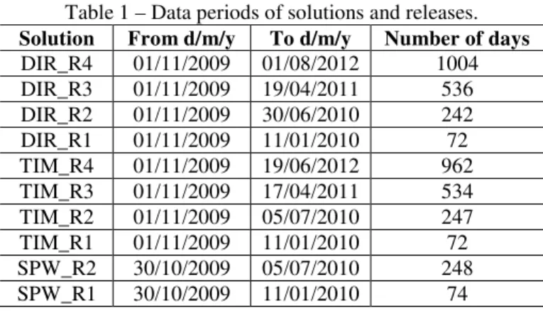
The State of São Paulo was chosen in order to compute the geo different techniques. Figure 1 presents the study area delimited b square. This area includes the State of São Paulo, as well as so surroundings, and extends from 26º–19º South in latitude and 54 longitude. The medium square represents the gravity data area and 28º–17º South in latitude and 56º–42º West in longitude. The larger the Digital Terrain Model (DTM) and the Digital Bathymetric Model is one degree larger than gravity area.
Figure 1 – Data area. Figure 2 – Terrestrial gra
4.1 Gravity Data Base
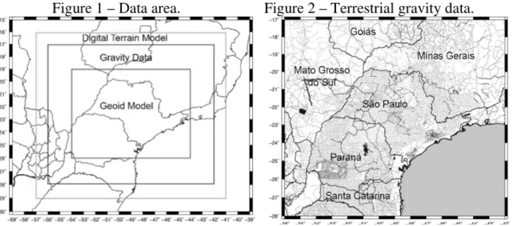
The gravity observations on land and sea represent the most esse information of the Earth’s gravity field and its internal density di terrestrial gravity observations carried out with absolute and relat form the basic data source for evaluating short wavelength of the E field (HECK, 1987).
In this paper, the Brazilian national gravity data set (BLITZKO was used. The study area consists of 46,290 stations (Figure 2) a provided by Observatório Nacional (ON), Brazilian Oil Company (P Instituto Brasileiro de Geografia e Estatística (IBGE), Instituto d Geofísica e Ciências Atmosféricas (IAG) and Escola Politécnica da de São Paulo (EPUSP). It is worth mentioning that FAPESP th contributed significantly towards the availability of the terrestrial gra especially in the State of São Paulo. Subsets also cover neighbo (Paraguay and Argentina). With an area of more than one million km large enough to provide feedback on the GOCE models. The ac Brazilian terrestrial gravity data is 0.1 mGal level or better (BLIT 2010). In some parts of the area, gravity data resolution is about 5-8 k Paraná and Santa Catarina states). In the northwest and northeast, th
odel in the State of...
eoid model using d by the smaller some of its and 54º–44º West in d it is limited by square is about del (DBM) and it
gravity data.
ssential source of distribution. The lative gravimeter e Earth’s gravity
Guimarães, G. N. et al. 1 9 1 about 10 km and there are some gaps. The gravity information was validated by a package dedicated to the validation of gravity data called DIVA developed by Bureau Gravimétrique International (BGI). In the ocean DTU10 (ANDERSEN, 2010) was used. This model is an update of DNSC08 (Danish National Space Center 2008) and it is a truly global gravity field with 1-2 km resolution grid.
4.2 Geopotential Models
The Global Gravitational Models expressed a substantial function in the geoid determination. They are responsible for the long wavelength information of the gravity field. In this paper, it was used GOCE-based models (discussed in the section 2) and EGM2008. Details concerning EGM2008 can be found in (PAVLIS et al., 2008) and (HOLMES; PAVLIS, 2008).
4.3 Digital Terrain Model
For the present study, a suitable gridded topography with a grid size of 3” x 3” (approximately 90 m x 90 m) from SAM3s_v2 (MATOS; BLITZKOW, 2008). This model consists of SRTM3 (FARR et al., 2007), but EGM96 (LEMOINE et al., 1998a and 1998b) geoid heights used in the SRTM3 was substituted by EIGEN-GL04C (FÖRSTE et al., 2006) in order to derive the orthometric height. Here the gaps were substituted by digitizing maps and DTM2002 (Digital Terrain Model 2002) topographic model (SALEH; PAVLIS, 2002). DTM2002 combines data from GLOBE (Global Land One-kilometer Base Elevation), version 1.0, constructed by the National Oceanic and Atmospheric Administration (NOAA) and the National Geophysical Data Center (NGDC) (HASTING; DUNBAR, 1999), and ACE (Altimeter Corrected Elevation), from Earth and Planetary Remote Sense Laboratory, University of Montfort, UK. In the ocean, the global model DTU10 was used (ANDERSEN, 2010).
4.4 GPS Leveling
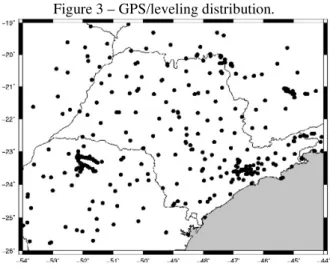
In this manuscript 363 GPS/leveling stations (Figure 3) was selected. The spirit leveling was carried out by the Brazilian surveying institute IBGE and the former IGG (Instituto Geográfico e Geológico), currently IGC (Instituto Geográfico e Cartográfico). The orthometric heights are referred to a local height datum (Imbituba tide gauge) and the ellipsoidal heights to WGS84 ellipsoid.
The computation of the geoid mo 1 9 2
Figure 3 – GPS/leveling distribution.
5 ESTIMATION PROCEDURES AND RESULTS
5.1 Geoid Model Computed by FFT
The schedule to determine the geoid model using FFT can be steps (BLITZKOW, et al. 2008):
1. Calculation of point free air gravity anomalies throu gravimetric data (coordinates, orthometric height and gravity 2. Calculation of complete Bouguer anomalies in order to de air gravity anomalies. The 5’ x 5’ grid of these anomalies from point gravity data. Over the ocean, DTU10 was used; 3. Calculation of Helmert gravity anomalies referred to the
Earth, which are obtained from the mean free air anomaly by Topographical Effect (DTE), Direct Atmospheric Effec Secondary Indirect Topographical Effect (SITE) (ELLMAN 2007);
4. Stokes’ integration with the use of the spectral decompositi the co-geoid. The modified Stokes’ kernel was computed Featherstone (2003);
5. Primary Indirect Topographical Effect (PITE) was adde heights to obtain geoid heights (MARTINEC; VANIČE
MARTINEC, 1998).
5.2 Geoid Model Computed by LSC
The methodology to compute the geoid using LSC is described bel
odel in the State of...
be described in 5
rough terrestrial ity acceleration); derive mean free es was computed
he surface of the by adding Direct fect (DAE) and AN; VANIČEK,
sition to calculate ted according to
ded to co-geoid
ČEK, 1994; and
Guimarães, G. N. et al. 1 9 3 1. Calculation of point free air gravity anomalies through terrestrial
gravimetric data (coordinates, orthometric height and gravity acceleration); 2. Use the remove-restore technique to remove the long-wavelength
component from the geopotential model and the residual terrain correction. Over the ocean, a refined DTM/bathymetry model (DTU10) is set up in order to estimate the RTC effect. This has been accomplished by merging the SRTM DTM with the available NOAA bathymetry of the Atlantic Ocean in the computation area;
3. Residual gravity anomaly interpolation in a 5’ grid;
4. Computation of the empirical and model covariance functions;
5. Computation applying the Fast Collocation method (BOTONI; BARZAGHI, 1993);
6. Restore the long-wavelength component and the residual terrain correction to obtain the geoid height.
5.3 Geoid Model Comparisons
Besides EGM2008, presented in figures and tables above, the geoid model was computed using GOCE-based models (DIR_R3 and TIM_R3), GOCO03S and EIGEN-6C in terms of long wavelength component. These geopotential models were chosen because they are the most recently available models. In the first comparison the geoid height residual difference was analyzed. In the second attempt, the differences between the geoid height provided by the geoid model and the geoid height obtained from GPS observations on Bench Marks of spirit leveling network were evaluated. This evaluation was undertaken in absolute way, while the third comparison was performed in relative way. Also a comparison involving only stations in the mountain area was performed in order to verify FFT and LSC behavior in this region.
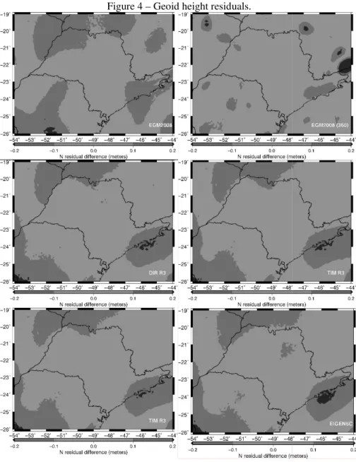
5.3.1 Geoid height residual comparisons
The geoid height residual was computed by the difference of FFT and LSC residual. This evaluation pretended to verify how is the compatibility of both methodologies in terms of short wavelength component. Figure 4 presents the differences.
The computation of the geoid mo 1 9 4
Figure 4 – Geoid height residuals.
Guimarães, G. N. et al. 1 9 5 Table 2 – Geoid height residual statistics.
GGMs
meters
Mean RMS
diff. Max. Min.
EGM2008 (150) 0.02 0.08 0.22 -0.25 EGM2008 (360) 0.01 0.06 0.49 -0.26 DIR_R3 (150) 0.02 0.08 0.24 -0.23 TIM_R3 (150) 0.02 0.08 0.23 -0.22 GOCO03S (150) 0.02 0.08 0.23 -0.22 EIGEN-6C (150) 0.02 0.08 0.24 -0.23
5.3.2 Absolute comparisons
The absolute comparison allows the analysis on how consistent is the geoid model and the GPS/leveling stations in relation to geoid height. The comparison between these two quantities has been performed in terms of root mean square difference. The absolute comparison statistics considering all GPS/leveling stations is presented in Table 3.
Table 3 – Absolute comparison statistics (units in meters).
Geoid Models Mean RMS diff. Max. Min.
FFT EGM2008 (150) 0.12 0.22 0.51 -0.43 FFT EGM2008 (360) 0.13 0.23 0.58 -0.41 LSC EGM2008 (150) 0.16 0.23 0.65 -0.36 LSC EGM2008 (360) 0.16 0.25 0.72 -0.47 FFT DIR_R3 (150) 0.11 0.21 0.49 -0.44 LSC DIR_R3 (150) 0.09 0.20 0.56 -0.50 FFT TIM_R3 (150) 0.11 0.22 0.51 -0.43 LSC TIM_R3 (150) 0.09 0.20 0.58 -0.47 FFT GOCO03S (150) 0.12 0.22 0.51 -0.43 LSC GOCO03S (150) 0.09 0.20 0.54 -0.47 FFT EIGEN-6C (150) 0.11 0.22 0.51 -0.45 LSC EIGEN-6C (150) 0.09 0.20 0.51 -0.49
Table 3 shows that both geoid models (using FFT and LSC) are consistent with GPS/leveling in relation to RMS difference. The differences vary between 0.20-0.22 m considering only the models up to degree and order 150. Results of geoid models based on GOCE data are slightly lesser than that based on EGM2008 data in terms of mean and RMS difference. The model computed by Least Squares Collocation presented more compatibility than Fast Fourier Transform when GOCE data were used.
The computation of the geoid mo 1 9 6
-0.40 m and 0.40 m) in the region close to the coast. Also, there are s scattered in some parts of the model. From 363 stations and consider evaluated, 55-65% of them have differences in the range from -0.20 40% between the range -0.21 to -0.40 m and 0.21 to 0.40 m and 5-10 m and 0.40 m.
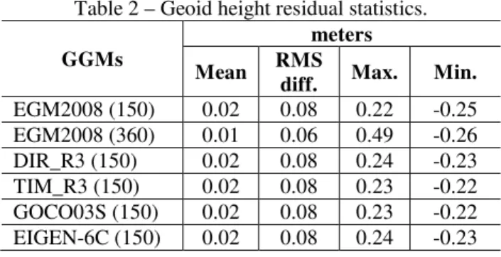
In order to evaluate only the State of São Paulo, some plots we GPS/leveling points interpolation to show the discrepancy throug (Figure 5).
Figure 5 – Discrepancy GEOID SP and GPS/leveling in the State o
odel in the State of... e some red points dering all models 20 to 0.20 m,
30-10% above -0.40
were made by the ughout the state
Guimarães, G. N. et al.
According to Figure 5, FFT and LSC have similar beh except for EGM2008, where LSC presented some dark spo especially in the mountain region. For the geoid models based behavior in terms of difference has the same standard.
1 9 7
The computation of the geoid mo 1 9 8
5.3.2.1 Absolute comparison in the mountains
In order to evaluate only GPS/leveling stations in the mountain were selected in this region (Figure 6). This evaluation pretends to sh behavior of both methodologies in a region with less gravity data tha of the state, since the highest differences, according to Figure 5, are in
Figure 6 – GPS/leveling stations in the mountain area.
Table 4 presents the evaluation for the referred area. Consideri the results using FFT are more consistent with GPS/leveling than LS RMS difference, the geoid model using EGM2008 presented the hig between FFT and LSC (0.05 m). The obvious conclusion for these that the covariance functions computed did not represent very well there is a lack of data and the topography is rugged. The compari height with the height anomaly is not an effective method for consistency of LSC and FFT techniques, in comparison with the technique, in order that anomalous masses, mainly in rugged topograp in a different way those two geodetic quantities.
Table 4 – Absolute comparison statistics in the mountains (units i
Geoid Models Mean RMS diff. Max.
FFT EGM2008 (150) 0.17 0.25 0.49 LSC EGM2008 (150) 0.25 0.30 0.59
FFT DIR_R3 (150) 0.17 0.24 0.47
LSC DIR_R3 (150) 0.22 0.26 0.56
FFT TIM_R3 (150) 0.18 0.25 0.50
LSC TIM_R3 (150) 0.23 0.28 0.58
FFT GOCO03S (150) 0.18 0.25 0.50 LSC GOCO03S (150) 0.22 0.27 0.51 FFT EIGEN-6C (150) 0.18 0.25 0.50 LSC EIGEN-6C (150) 0.22 0.27 0.51
odel in the State of...
in area, 83 points show how is the han in other parts e in this area.
ea.
ering all models, LSC. In terms of highest difference ese differences is ll this area, since arison of geoidal or analyzing the the leveling/GPS raphy area, affect
ts in meters).
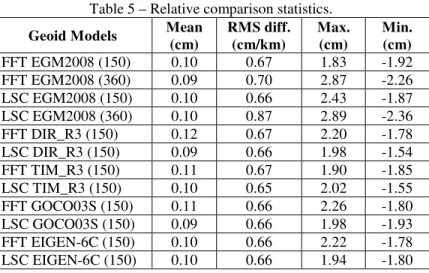
Guimarães, G. N. et al. 1 9 9 5.3.3 Relative comparisons
In relative comparison, pairs of points spaced among 20 – 50 km were selected. This range allows evaluating the influence of short wavelength component. A total of 135 pairs were selected. The standard difference value was defined as the mean value resultant of all bases. In this case, EGM2008 up to degree and order 150 was used as reference field. Table 5 presents the relative comparison statistics.
Table 5 – Relative comparison statistics.
Geoid Models Mean
(cm)
RMS diff. (cm/km)
Max. (cm)
Min. (cm)
FFT EGM2008 (150) 0.10 0.67 1.83 -1.92 FFT EGM2008 (360) 0.09 0.70 2.87 -2.26 LSC EGM2008 (150) 0.10 0.66 2.43 -1.87 LSC EGM2008 (360) 0.10 0.87 2.89 -2.36
FFT DIR_R3 (150) 0.12 0.67 2.20 -1.78
LSC DIR_R3 (150) 0.09 0.66 1.98 -1.54
FFT TIM_R3 (150) 0.11 0.67 1.90 -1.85
LSC TIM_R3 (150) 0.10 0.65 2.02 -1.55
FFT GOCO03S (150) 0.11 0.66 2.26 -1.80 LSC GOCO03S (150) 0.09 0.66 1.98 -1.93 FFT EIGEN-6C (150) 0.10 0.66 2.22 -1.78 LSC EIGEN-6C (150) 0.10 0.66 1.94 -1.80
The statistics in Table 5 shows that the comparison for the geoid models up to degree and order 150 are very similar. Regarding the maximum and minimum, FFT models presented higher values than LSC models. This shows that the influence of the short wavelength component of all models have the same behavior in terms of mean and RMS.
6. CONCLUSIONS
The geoid model in the State of São Paulo was computed using two different methodologies (Stokes’ integral applying Fast Fourier Transform and Least Squares Collocation). The computation was performed using EGM2008 (degree and order 150 and 360), GOCE-based models (DIR_R3 and TIM_R3), GOCO03S and EIGEN6C (degree and order 150) as the reference field for long wavelength component. Three comparisons were carried out to verify the quality and consistency of the models. In the first evaluation, the geoid height residual computed by FFT and LSC was compared for the same degree and order. Regarding all geoid models, for n=m=150, 65-70% of the area has differences between 0.00 m and M 0.10 m, 30-35% between M 0.10 m and M 0.20 m and 0.40-1.00% larger than
The computation of the geoid model in the State of... 2 0 0
m and 1.00% larger than M 0.20 m. In this case, differences larger than 0.20 m were found in the places that there are some gaps in terms of gravity data. It can be concluded that in the most part of the State of São Paulo both methodologies are consistent in the order of 0.10 m.
In the second comparison, the geoid models were verified by comparing GPS/leveling points in the absolute way. This is a very powerful tool to analyze the consistency of each other. It was used 363 points distributed all over the area. The differences in terms of root mean square are between 0.20 m and 0.23 m for models up to 150. The geoid models based on GOCE data presented better consistency with GPS/leveling points than EGM2008. Furthermore, LSC models fitted better than FFT for the GOCE models. However, in the absolute comparison in the mountains, FFT is more consistent than LSC. In this case, the RMS differences for the geoid models using FFT are between 0.24 m and 0.25 m, while the LSC models are between 0.26 m and 0.30 m. The reason for LSC be less compatible than FFT can be explained by the lack of data and the topography that affected the LSC computation, since the gravity anomalies are highly correlated with the topography and can influence the modeling of covariance functions. Again, the models based on GOCE data presented similar results in relation to EGM2008 in the mountain area. In the third evaluation, relative comparisons showed that FFT and LSC (n=m=150) presented very close results. In terms of RMS, the differences are between 0.65 and 0.67 cm/km.
It is worth mentioning that a study in terms of tide system should be carried out, since the spirit leveling network is referred to the mean tide and the geopotential models are tide free. Also, it is important to cover the lacks of gravity data in the State of São Paulo and surrounding area. In this way, the geoid model would be improved. The geoid model computation in an area with poor gravity data distribution could be an opportunity to verify the LSC methodology and also the covariance functions. LSC could be tested in the Amazon region. In most part of the forest there is no gravity data, however, close to the rivers there are a substantial quantity of data. Furthermore, this region is quite flat, which could be a positive indication in determining the covariance functions. The use of GPS and gravity data in the LSC determination could be undertaken to verify how GPS can contributes in the geoid model computation.
ACKNOWLEDGEMENTS
The first author acknowledgement CAPES and CNPq agencies for the granting of the scholarship and the university Politecnico di Milano by hosting for one year during the doctorate studying.
Guimarães, G. N. et al. 2 0 1
REFERENCES
ANDERSEN, O.B. The DTU10 Gravity field and Mean sea surface. Second International Symposium of the Gravity Field Service – IGFS2 20 – 22 September 2010 Fairbanks, Alaska, 2010.
BLITZKOW, D.; et al. An attempt for an Amazon geoid model using Helmert gravity anomaly. In: Michael G. Sideris. (Org.). Observing our Changing Earth. 1 ed. : Springer-Verlag, 2008, v. 133, p. 187-194, 2008.
BLITZKOW, D.; et al. A new version of the geoid model for South America. Second International Symposium of the International Gravity Field Service – IGFS2 20 – 22 September 2010 Fairbanks, Alaska, 2010.
BOTTONI, G.P.; BARZAGHI, R. Fast collocation. Bulletin Géodésique. v. 67, p. 119-126, 1993.
BRUINSMA, S.L.; et al. GOCE gravity field recovery by means of the direct numerical method, presented at the ESA Living Planet Symposium, 27th June - 2nd July, Bergen, Norway, 2010, See also: earth.esa.int/GOCE.
DRINKWATER, M.R.; et al. The GOCE gravity mission: ESA’s first core earth explorer, Proceedings… of 3rd International GOCE User Workshop, 6-8 November, 2006, Frascati, Italy, ESA SP-627, ISBN 92-9092-938-3, p.1-8, 2007.
ELLMANN, A.; VANÍČEK, P. UNB applications of Stokes-Helmert’s approach to
geoid computation. Journal of Geodynamics, v. 43, p. 200-213, 2007.
ESA – ESA’s gravity mission – GOCE. BR-2009. Revised June 2006. ESA Publications Division. ESTEC, Noordwijk, The Netherlands, 2006.
FARR, T.G.; et al. The Shuttle Radar Topography Mission, Reviews of Geophysics, v. 45, 2007, DOI:10.1029/2005RG000183.
FEATHERSTONE, W.E. Software for computing five existing types of deterministically modified integration kernel for gravimetric geoid determination. Computer & Geosciences, v. 29, p. 183-193, 2003. Software available at: http://www.iamg.org/CGEditor/index.html
FÖRSTE C.; et al. A mean global gravity field model from the combination of satellite mission and altimetry/gravimetry surface data – EIGEN-GL04C, Geophysical Research Abstracts, v. 8, 2006.
GRACE – Gravity recovery and climate experiment: Science and mission. Requirements document, revision A, JPLD-15928, NASA’s Earth System Science Pathfinder Program, 1998.
HASTING, D.A.; DUNBAR, P.K. Global land one-kilometer base elevation (GLOBE) Digital Elevation Model Documentation, v 1, National Oceanic and Atmospheric Administration, National Geophysical Data Center, 1999. HECK, B.; GRÜNINGER, W. Modification of Stokes’ integral formula by
combining two classical approaches. Poster Presentation in IUGG General Assembly, Vancouver, 1987.
The computation of the geoid model in the State of... 2 0 2
HOLMES, S.; PAVLIS, N.K. Earth Gravitational Model 2008 (EGM2008).
Available in: http://earthinfo.
nga.mil/GandG/wgs84/gravitymod/egm2008/first_release.html. Access in: October 2012.
IBGE. Ajustamento simultâneo da rede altimétrico de alta precisão do sistema brasileiro geodésico brasileiro. Relatório, Rio de Janeiro, 62p. Available in: <http://www.ibge.gov.br/home/geociencias/geodesia/altimetrica.shtm> access in October 2011.
LEMOINE, F.G.; et al. New high-resolution model developed for Earth' gravitational field, EOS, Transactions AGU, 79, 9, March 3, v. 113, p. 117-118. 1998a.
LEMOINE, F.G.; et al. The development of the joint NASA GSFC and the National
Imagery and Mapping Agency (NIMA) geopotential model EGM96,
NASA/TP-1998-206861. National Aeronautics and Space Administration, Maryland, USA. 1998b.
LOBIANCO, M.C.B. Determinação das alturas do geoide no Brasil. 2005. 165p. PhD Thesis – Escola Politécnica da Universidade de São Paulo, São Paulo, 2005.
MATOS, A.C.O.C.; BLITZKOW, D. Modelagem Digital de Terrenos (MDT) de 3" para a América do Sul Pos-Doc Report – Escola Politécnica, Universidade de São Paulo, São Paulo, 2008.
MARTINEC, Z. Effect of lateral density variations of topographical masses in view of improving geoid model accuracy over Canada. Final Report of the contract DSS No. 23244-2-4356. Geodetic Survey of Canada, Ottawa, 1993.
MARTINEC, Z. Boundary-value problems for gravimetric determination of a precise geoid. Lecture Notes in Earth Sciences, v. 73, 1998.
MARTINEC, Z.; VANÍČEK, P. Direct topographical effect of Helmert's
condensation for a spherical approximation of the geoid. Manuscripta Geodaetica, n. 19, p. 257-268, 1994.
MEISSL, P. Preparations for the numerical evaluation of second-order
Molodenskii-type formulas. Columbus, Dep. of Geodetic Science and
Surveying. Ohio State University, Report 163, 1971.
MIGLIACCIO, F.; et al. GOCE data analysis: the space-wise approach and the first space-wise gravity field model. Proceedings of the ESA Living Planet Symposium, 28 June - 2 July 2010, Bergen, Norway, 2010.
MORITZ, H. Advanced physical geodesy, 2nd Edition, Karlsruhe: Wichmann, 1989. NOVÁK, P. Evaluation of gravity data for the Stokes–Helmert solution to the
geodetic boundary-value problem. Technical Report No. 207, Department of Geodesy and Geomatics Engineering, University of New Brunswick, Fredericton. 2000.
Guimarães, G. N. et al. 2 0 3
Symposium, 28 June - 2 July 2010, Bergen, Norway, See also:
earth.esa.int/GOCE. 2010.
PAVLIS, N.K. Global gravitational modeling & development and applications of geopotential models. (An overview considering current and future dedicated gravity mapping missions) Lectures notes for the Ninth International School for the Determination and use of the Geoid. La Plata, Argentina, 2010.
PAVLIS, N.K.; et al. An Earth gravitational model to degree 2160: EGM2008. presented at the 2008 General Assembly of the European Geosciences Union, Vienna, Austria, April 13-18, 2008.
RAPP, R.H. Past and future developments in geopotential modeling, geodesy on the move. Forsberg, Feissel, Dietrich (eds), Springer-Verlag Berlin. New York, p. 58-78,1998.
REIGBER, C.; et al. CHAMP phase-B executive summary. GFZ, STR96/13, 1996. SÁ, N.C.; VIEIRA, C. Rede GPS do estado de São Paulo: aprimoramento de
modelos geoidais e apoio básico local. Relatório científico final FAPESP (Processo: 99/012691-9) Instituto de Astronomia, Geofísica e Ciências Atmosféricas, Universidade de São Paulo, São Paulo, 90p, 2006.
SALEH, J.; PAVLIS, N.K. The development and evaluation of the global digital terrain model DTM2002. Presented at the 3rd Meeting of the International Gravity and Geoid Commission, Thessaloniki, Greece 26 - 30 August 2002. TSCHERNING C.C. Collocation methods in harmonic spaces. Proceedings… of the
Free Boundary Value Problems Meeting. Born, 1971.
TSCHERNING C.C.; RAPP, R.H. Closed covariance expressions for gravity anomalies, geoid undulation and deflections of the vertical implied by the anomaly degree covariance models. Report of the Ohio State University. Columbus, n. 208, 1974.
VANÍČEK, P.; KLEUSBERG, A. The Canadian geoid - Stokesian approach.
Manuscripta Geodaetica, v. 12, p. 86-98, 1987.
VANÍČEK, P.; et al. Determination of the boundary values for the Stokes-Helmert
problem. Journal of Geodesy, v. 73, p. 160-192, 1999.
VISSER, P.N.A.M.; VAN DEN IJSSEL, J; KOOP, R.; KLEES, R. Exploring gravity field determination from orbit perturbations of the European Gravity Mission GOCE. Journal of Geodesy, v. 75, p. 89-98, 2001.