Quim. Nova, Vol. 35, No. 1, 45-50, 2012
Artigo
*e-mail: [email protected]
ORGANIC AND TOTAL MERCURY DETERMINATION IN SEDIMENTS BY COLD VAPOR ATOMIC
ABSORPTION SPECTROMETRY: METHODOLOGY VALIDATION AND UNCERTAINTY MEASUREMENTS
Robson L. Franklin*
Laboratório de Química Inorgânica, Companhia Ambiental do Estado de São Paulo, Av. Frederico Hermann Jr., 345, 05459-900 São Paulo - SP, Brasil
Jose E. Bevilacqua
Diretoria de Tecnologia, Qualidade e Avaliação Ambiental, Companhia Ambiental do Estado de São Paulo, São Paulo / Centro de Estudos Químicos, Centro Universitário FIEO, Av. Franz Voegeli, 300, 06020-190 Osasco – SP, Brasil
Deborah I. T. Favaro
Instituto de Pesquisas Energéticas e Nucleares, Av. Prof. Lineu Prestes, 2242, 05508-000 São Paulo – SP, Brasil
Recebido em 10/1/11; aceito em 1/6/11; publicado na web em 22/7/11
The purpose of the present study was to validate a method for organic Hg determination in sediment. The procedure for organic Hg was adapted from literature, where the organomercurial compounds were extracted with dichloromethane in acid medium and subsequent destruction of organic compounds by bromine chloride. Total Hg was performed according to 3051A USEPA methodology. Mercury quantification for both methodologies was then performed by CVAAS. Methodology validation was verified by analyzing certified reference materials for total Hg and methylmercury. The uncertainties for both methodologies were calculated. The quantification limit of 3.3 µg kg-1 was found for organic Hg by CVAAS.
Keywords: sediments; organic mercury; CVAAS.
INTRODUCTION
Mercury is one of the most hazardous environmental pollutants and exists in a large number of physical and chemical forms with a large variety of properties that determine its complex distribution, biological enrichment and toxicity.1 Although all forms of mercury
are poisonous, the ecological and human health effects are generally related to the environmental transformations of mercury into the toxic and biomagnification-prone compound methylmercury (MeHg).2 The
methylation and demethylation processes often occur in sediments. This compartment acts as the source for mercury methylation, which subsequently leads to bioaccumulation.3 Therefore, the accurate and
precise determination of MeHg in sediments is a key point to better understand the biogeochemical cycling of this contaminant and to estimate the associated exposures.
The organomercurial compounds are potentially more toxic than the inorganic forms of Hg, being methylmercury (MeHg) the compound present in greater amounts than other organic forms in the sediments, representing about 90% or more of these organic forms, depending on geochemical characteristics of the sediments. 4-8
Ethyl and methylmercury affects the central nervous system and depending on the exposure time, symptoms may be irreversible and can eventually lead to death.6-9
The term organic Hg has been used to include all the organomer-curial compounds that are found in environmental samples such as methylHg, dimethylHg and phenylHg.
As other organometallic species, the analytical methods used for MeHg determination in sediments involve many steps. First, the solid sample must be extracted to secure the integrity of the mercury species present in the sample. Then, mercury species are separated and usually detected by atomic spectrometry (CVAAS and CVAFS) or mass spectrometry (GC-MS or ICP-MS) with or without a previous
preconcentration step. Different combinations of steps have been reviewed recently.10-12 However, such methods require sophisticated and costly equipment for an efficient separation and reliable quanti-fication of organomercurial compounds.
Unfortunately, many Brazilian research centers and laboratories are not adequately structured for organomercurials quantification in geological samples. A simpler and cheaper CVAAS instrumentation along with an analytical procedure adapted for organomercurial compound analyses is a possible solution for organomercurial quantification in contaminated samples. Furthermore, INMETRO requires statistical tools such as uncertainty measurements for ABNT ISO 17025 laboratory accreditation. This accreditation certifies the laboratory as having the necessary scientific technical requirements.
The purpose of the present study was to adapt the methodology described by Bisinoti et al.13 based on the extraction of organic
EXPERIMENTAL
Organic mercury determination procedure
The analytical method used for organic Hg quantification was adapted with some modifications from Bisinoti et al.13 and based
on the extraction of organic Hg forms with dichloromethane and hydrochloric acid. Modifications consisted in altering the quantity and concentration of HCl used in the extraction step. Bisinoti used 5.0 mL of HCl 6.0M whereas this study used 15.0 mL of HCl 2.0M. This alteration was done in order to avoid the accidental formation of organomercurial compounds that can occur in higher concentrations of HCl in samples characterized by high organic matter and high inorganic Hg contents.12,14,15 In the present study the preliminary
results using BCR CRM 580 and IAEA 405 reference materials, the organic concentrations found were much higher than the certified values using 5 mL of HCl 6.0 M. IAEA 405 showed a variation of 9 to 12 µg kg-1 when compared to the 5.5 µg kg-1 certified value. For
BCR CRM 580 the values fell between 97 and 115 µg kg-1, the
certi-fied reference value being 75 µg kg-1. The chemical recoveries were
between 130 and 220% interval range. EPA16 acceptance criteria vary
from 65 to 135% for aqueous solutions. Does the reduction of HCl concentration from 6 to 2 M while maintaining the molar amount of HCl in the extraction and increasing the volume of HCl used from 05 to 15 mL was chosen.
A further alteration was to use a CVAAS detection system instead of CVAFS, more commonly found in Brazilian laboratories; however this change reflects the inability of quantifying the analyte in low concentrations. About 1.0 to 2.0g of reference material or sample was weighed in glass flasks to which 15 mL of 2.0 mol L-1 HCl
(Merck) was added and put in an ultra-sound bath for 15 min. After this, 15 mL of dichloromethane was added and the mixture agitated for at least 12 h at 150 rpm. The sample was then filtered using glass wool (CAAL) (previously treated with dichloromethane, HCl and deionized water, and heated in an oven), in order to separate sediment from its liquid phase. Centrifugation can be also used for this purpose. After this step, the dichloromethane phase was separated from the HCl phase in a separatory funnel. To the dichloromethane phase, containing all the organic compounds extracted from the sediments including all organomercurial compounds, 30 mL of 3.0% (v,v) HNO3 (Merck) was added. This mixture was bubbled with ultrapure
N2 gas (ECD level, from White Martins) for 20 min, approximately,
and transferred to a 50 mL volumetric flask. To this flask, 400 µL of bromine chloride solution (1.50 g of KBr (Merck) and 0.58 g of KBrO3 (Merck) in 100 mL conc. HCl) was added and after 30 min,
800 µL of 30% hydroxylamine hydrochloride (Carlo Erba). Volume was completed to 50 mL with deionized water and again put in an ultra-sound bath for 10 min. Hg determination was then performed by CVAAS using FIMS (Flow Injection Mercury System) from Perkin Elmer and stannous chloride 1.1% (m,v) (Merck) as a reducing agent. Total mercury determination procedure
About 0.5g of reference material was weighed directly in Teflon tubes, 10 mL of conc. HNO3 (Carlo Erba) was added and digestion
carried out according to method EPA 3051A17 and put into 50 mL
volumetric flask. Total Hg determination was performed by CVAAS using FIMS from Perkin Elmer and 1.1% (m,v) stannous chloride as a reducing agent.
Calibration curve
The calibration curve used for total and organic Hg quantification
was prepared daily from a standard solution (Merck) traceable to NIST (National Institute of Standards and Technology, USA).
The micropipettes and the volumetric flasks used for preparation of intermediate standard solutions were calibrated by RBC (Rede Brasileira de Calibração). Table 1 presents the data of the calibration curve prepared. (y = 69.87286*x – 0.00388, with correlation coeffi-cient = 0.99967) by using FIMS from Perkin Elmer.
The calibration curves were prepared daily and two readings of each concentration value were taken. The calibration curve pre-sented (Table 1) was that used for the calculations of quantification and detection limits. The minimum correlation coefficient value of 0.998 was the acceptance criterion for the calibration curves, with a confidence level of 95%.
The “expected concentration” column presents the concentration of the prepared solutions with their respective uncertainties, while “calculated concentration” column presents the values obtained from the instrument calibration.
Three standard control solutions (1.021 ± 0.055; 2.552 ± 0.074; 4.082 ± 0.099, in this day), prepared and calculated daily, from another standard solution from Accustandard also traceable to NIST standard solution were used to confirm the concentration of the calibration curve. All solutions prepared for the calibration curve as well as standard control solutions were prepared in the same manner as the samples were, including the digestion procedure assisted by micro-wave oven in acid media in closed vessel, according to EPA 3015A.18
Detection (DL) and quantification (QL) limits for total Hg determination
Detection and quantification limits were determined taking into account the analytical curve (Table 1).
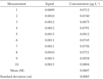
These limits were determined in the presence of analyte. The standard deviation is calculated as the lowest concentration of the analyte measurable by the analytical method. The detection limit is considered as three times the standard deviation value and the quantification limit, as ten times the standard deviation. To obtain this standard deviation value a three times dilution of the lowest concentration point in the calibration curve was made and the deter-mination was performed immediately after dilution. The results are presented in Table 2.
As the acceptance criterion, the value of ten times the standard deviation (10*sd) must be higher than the mean of the individual measurements. In this case the detection limit was calculated as being 3* 0.0085 = 0.0256 ≈ 0.03 µg L-1. The quantification limit
was calculated as being ten times the standard deviation (10* 0.0085 = 0.085 µg L-1), considering 0.10 µg L-1 as the DL value merely as
a safety margin.
In the case of sediment samples prepared according to the US EPA procedure,17 a dilution factor of about 100 (0.5 g of sample in Table 1. Analytical curve prepared from Hg standard calibration solutions
Point Expected concentration
(µg L-1)
Calculated concentration (µg L-1) Calibration blank 0.00
S1 0.253 ± 0.012 0.2495
S2 0.506 ± 0.029 0.4896
S3 2.539 ± 0.067 2.618
S4 5.036 ± 0.090 5.134
50 mL volumetric flask) should be considered. This means that the quantification limit for total Hg in sediment samples is 10 µg kg-1
or 0.01 mg kg-1.
Detection (DL) and quantification (QL) limits for organic Hg determination
In this case, besides the DL and QL calculation for total Hg de-termination, one has to consider that the analytical procedure started with 1.5 g of sediment sample and final volume of 50 mL, giving a dilution factor of 33. Therefore, for organic Hg determination in sediments, the LQ is 33*0.10 = 3.3 µg kg-1. Calculation was performed
considering a wet sample. On a dry basis the LQ will be 10 µg kg-1,
for a sample with 70% humidity.
Uncertainty assessment for total Hg determination
The acceptable interval presented in Table 3 corresponds to the standard uncertainty (u) of these standard control solutions. The uncer-tainty assessment of a sample is defined as a parameter associated to the result of a measurement that characterizes the dispersion of values that can be fundamentally attributed to a measurand.19 The uncertainty
assessment can be calculated from the known standard uncertainties of all factors of variability that influence the measurement. For instance, uncertainty of the standard solution given by the manufacturer, uncer-tainty of micropipette used in the solution preparation, unceruncer-tainty of the volumetric flask and the calibration of its volume, etc.
According to INMETRO,20 the combined standard uncertainty
“uc” can also be calculated from the square root of the sum of all
variances of the process. Then the expanded uncertainty “U”, for a 95% significance level, can be obtained multiplying the combined uncertainty ‘uc” by an abrangency factor (k) of 2.
The analytical method for total Hg determination by CVAAS at CETESB has been assessed for all the parameters described above.
All the process and methodology variabilities were taken into account considering the variability of the last hundred values obtained for each one of the parameters, involving, among others, the uncertain-ty of the calibration standards. Thus, for calculation of combined uncertainty of the analytical results for total Hg determination in the present study, the relative standard deviation obtained from the mean of replicates and uncertainty measured from standard control solutions, are considered in the Equation 1:
uC = √sd
2 + ic2 (1)
and U = k uc
where: uc – standard combined uncertainty; sd – standard deviation
of the sample analysis; ic –combined uncertainty of the procedure
obtained by means of the standard control solutions.
The contribution ic is the mean of the uncertainties of the method
calculated from historical data from standard control solutions, which is, 0.22 µg L-1, and includes the uncertainty of calibration standard. This uncertainty value is practically linear for the constructed ca-libration curve. The uncertainty value for the 1.00 µg L-1concentration value is that of 0.160 µg L-1. For the 2.50 µg L-1 concentration value the calculated uncertainty is 0.179 µg L-1 and for 4.00 µg L-1, 0.216 µg L-1. The greater uncertainty value (0.216 µg L-1) was adopted for all quantification ranges.
The uncertainty of the analytical curve (that obtained from Table 1), whose calculations were performed by means of the mi-nimum squares (0.044 for the highest concentration point) can be considered low when compared to the value obtained by the standard control solutions concentration variations and can be eliminated in Equation 1 and adopting this procedure it should be noted that the measurement of uncertainty near the method´s quantification limit may be overestimated.
Therefore, the value of uncertainty calculated for total Hg will be the combination of the analytical methodology uncertainty con-sidering the historical data of the standard control solutions with the standard deviation of replicates of sample analyses.
Uncertainty for the organic Hg determination
For calculation of the uncertainty in the organic Hg determina-tion procedure, besides the contribudetermina-tions already described for total Hg determination, there is one more variable and difficulty in the process this being the organic extraction phase. In this step various factors contribute for the uncertainty measurement, such as solvent partition coefficients, small temperature oscillations, vapor pressure of analyte and solvents, among others. Due to the complexity of the analytical procedure, mainly for identification and calculation of uncertainty sources in the organic extraction step, the uncertainty estimate was calculated by using the standard deviation (%) in the reference material analyses, according to INMETRO.20 For the IAEA
405, the certified value for MeHg is 5.49 ± 0.53 µg kg-1 and for BCR
580, 75 ± 4 µg kg-1. These values are related to the MeHg content and
not to the organic Hg. The organic Hg concentration obtained by this procedure will always be higher or similar to the MeHg concentration.
Table 2.Standard deviation of the lowest concentration determination of the analite (total Hg) (n=10)
Measurement Signal Concentration (µg L-1)
1 0.0009 0.0712
2 0.0010 0.0740
3 0.0012 0.0875
4 0.0012 0.0791
5 0.0013 0.0912
6 0.0011 0.0745
7 0.0011 0.0756
8 0.0010 0.0721
9 0.0013 0.0928
10 0.0013 0.0894
Mean (M) 0.0807
Standard deviation (sd) 0.0085
Table 3. Results for the standard control solutions prepared as control in order to check the calibration curve (Table 1)
Expected concentration ± uncertainty (µg L-1)
Calculated concentration by FIMS ± uncertainty (µg L-1)
Acceptance interval
Control 1 1.021 ± 0.055 1.030 ± 0.223 0.862 - 1.181
Control 2 2.552 ± 0.074 2.548 ± 0.230 2.374 - 2.730
The expression for uncertainty estimation in the organic Hg determination will be described in Equation 2:
uC = √sd
2 + ((mdmr/100)
*Vl)2 + ic2 (2) and U = kuc
being: uc – standard combined uncertainty for organic Hg
determi-nation; sd – standard deviation of the sample determidetermi-nation; mdmr – mean value of the standard deviation for the reference material analyses; Vl – determined value; ic – uncertainty combined for the
methodology obtained through the mean of standard control solutions (already described).
The “mdmr” variable is a major contributor for the calculated uncertainty here presented. Its calculation is presented below. RESULTS AND DISCUSSION
Standard control solutions presented the results shown in Table 3. The acceptance interval for standard control solutions represents the standard uncertainty of these solutions, calculated according to INME-TRO20 and is based on a confidence level of 95%. In the first column of
Table 3, the value and uncertainty expressed is of that of the solution preparation. The second column is obtained from the equipment with the combined uncertainty calculated according to Equation 1.
The results obtained through the standard control solutions within the acceptance interval indicated that the equipment was capable of quantifications within the constructed analytical curve (Table 1).
Blanks were analyzed (n=3) not only for total Hg quantification, but organic Hg as well. Both were prepared or extracted in the some way of the standard. Blank results for total Hg ranged from 0.007 to 0.012 µg L-1 and to organic Mercury between 0.01 a 0.02 µg L-1.
The analytical methodology for Hg speciation (in organic mer-cury and inorganic mermer-cury) in environmental samples developed in this study can be applied in laboratories without any sophisticated equipment for Hg determination, only a CVAAS is needed. The QL obtained by using this analytical method (3.3 µg kg-1) is not too low when compared to literature values but it can be easily employed in sediment samples which are contaminated with Hg.
Analytical quality control (AQC) for the assessment of trueness of the analytical result
Reference material analyses was performed in the BCR CRM 580 (total and methylmercury in estuarine sediment)and IAEA 405 (estuarine sediment) reference materials for both, total and organic Hg in order to verify the accuracy of both analytical methods. The results obtained for all determinations of reference materials are shown in Tables 4 and 5. The recovery factors were 96.3 % for total Hg (0.78 ± 0.07 mg kg-1) and 106.6% for MeHg (5.8 µg kg-1± 1.0 as
sd) determined as organic Hg for the IAEA 405 and 96.2% for the total Hg (127 ± 7 mg kg-1) and 84.8% (64 µg kg-1 ± 13, as sd), for
the BCR CRM 580.
As we can observe the chemical recovery for the BCR CRM 580 reference material ranged from 64.1 to 112.3%. The mean value obtained for 11 determinations for organic Hg was lower than the certified value (75 ± 4 µg kg-1), showing a relative standard deviation
of 20.9% and relative error of 15.2%.
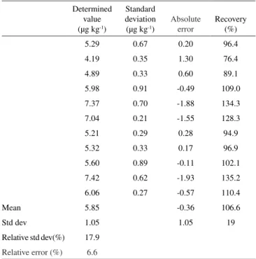
For the IAEA 405 reference material, the chemical recovery ranged from 76.4 to 135.2% and the mean value for 11 determina-tions of organic Hg was higher than the certified value (5.49 ± 0.53 µg kg-1), showing a relative standard deviation of 17.9% and relative
error of 6.6%.
As acceptance criteria of recovery percentages were those
recog-nized by the US EPA16 for spike in aqueous solutions which define
an acceptable range between 65 and 135% of recovery. Interference assessment in the organic Hg extraction
Inorganic Hg
Methylmercury chloride solution (Aldrich) was prepared in se-veral concentrations (in µg L-1) in 1.0 to 5.0 mg L-1 of inorganic Hg
solutions (Accustandard). MeHg was determined using the analytical procedure for organic Hg determination in order to verify if the me-thod could also transfer some inorganic Hg. The results obtained are shown in Table 6 andcorrespond to an average recovery of 97.8%.
Table 4. Results for organic Hg in BCR CRM 580 (75 ± 4 µg kg-1 as Me Hg)
Determined Value (µg kg-1)
Standard deviation (µg kg-1)
Absolute error
Chemical recovery(%)
77.9 0.6 -2.9 103.9
84.2 0.4 -9.2 112.3
60.5 0.7 14.5 80.7
48.5 0.6 26.5 64.7
53.3 1.1 21.8 71.0
74.5 0.6 0.5 99.4
48.3 1.3 26.7 64.3
58.7 0.4 16.3 78.3
48.0 3.5 27 64.0
70.3 0.2 4.7 93.8
75.4 3.9 -0.4 100.5
Mean 63.6 11.4 84.8
Std dev 13.3 13.3 17.8
Relative std dev (%) 20.9
Relative error (%) 15.2
Table 5. Results for organic Hg in the IAEA 405 reference material (5.49 ± 0.53 µg kg-1 as MeHg)
Determined value (µg kg-1)
Standard deviation (µg kg-1)
Absolute error
Recovery (%)
5.29 0.67 0.20 96.4
4.19 0.35 1.30 76.4
4.89 0.33 0.60 89.1
5.98 0.91 -0.49 109.0
7.37 0.70 -1.88 134.3
7.04 0.21 -1.55 128.3
5.21 0.29 0.28 94.9
5.32 0.33 0.17 96.9
5.60 0.89 -0.11 102.1
7.42 0.62 -1.93 135.2
6.06 0.27 -0.57 110.4
Mean 5.85 -0.36 106.6
Std dev 1.05 1.05 19
Relative std dev(%) 17.9
Blank analyses indicated Hg concentration levels below 0.1 µg L-1.
No inorganic Hg transfer was observed.
The approximate 10 µg L-1 concentration was chosen randomly.
This experiment was carried out only to verify any possible inorganic Hg methylation during the extraction process.
The standard deviation values obtained in the reference material analyses and the MeHg chloride recoveries in relation to the absolute value compose the variable “mdmr” in Equation 2, used to determine the uncertainty assessment for organic Hg quantification in this study. Looking again at Equation 2 for uncertainty calculation, the variable “ic” has a fixed constant value of 0.22 µg L-1. The value for
“mdmr” variable for Equation 2, is the square root of the sum of all standard deviation values obtained for the reference material analyses and MeHg chloride standard or
√1,052 + 1,172 + 13,342 = 13,4 µg L-1 (2)
The results shown in Table 4 to 6 confirm the validation of the analytical procedure used for extraction of organic Hg from sedi-ments. The mean recovery (%) in the reference material analyses as well as MeHg chloride determination (84 to 112%) were both within the acceptable range recommended by the US EPA according to the 1630 method16 for the extraction of standard additions of MeHg in
aqueous matrices. US EPA defined the ideal recovery as being betwe-en 65 and 135%, with the maximum standard deviation of 31%. There were some recovery values below 65% for the reference material BCR CRM 580 (64.0 and 64.7 %). These values were considered acceptable due to the fact that the criteria have been established for aqueous solutions and not for sediments. It is important to note that this procedure is related to organic Hg determination.
These results also indicate that the methodology is within the ac-ceptable ranges in regards to accidental methylation which can occur when analyzing organomercurial compounds. Several authors11-15, 21-24
cite the accidental MeHg formation as one of the main problems in determining this analite and consequently in the organic Hg determi-nation. According to these authors, the % of Hg+2 methylated is low
(up to 0.5%, but normally between 0.01 to 0.05% in relation to Hg+2).
The positive error in the MeHg concentration due to this effect is important only when the relationship between MeHg and inorganic Hg in the sample is < 1%. This occurs in some polluted sediments and residual waters, depending on the quantity of Hg+2 and
methyla-tion potential of the sample, which also depends mainly on organic matter content.12,14,15,22,23 Then the methylation contribution was not
considered in this study once is too low.
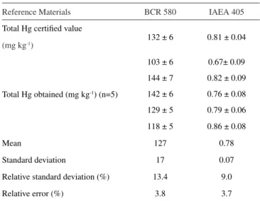
Table 7 presents the results obtained in the reference material analyses for total Hg using the experimental procedure according to the US EPA 3051A.
The recovery factors for total Hg were 96.2% for the BCR CRM 580 (127 ± 17 mg kg-1) and 96.3% (0.78 ± 0.07 mg kg-1) in the IAEA
405. The relative standard deviation was 13.4 and 9.0% and bias, 3.8 and 3.7%, respectively, showing the accuracy of the analytical methodology.
CONCLUSIONS
The analytical method used for organic Hg determination proved to be efficient and was validated by the results of the reference mate-rial analyzed. The methodology showed no analite in the blanks and resulted in good standard deviation values (< 20%).
The method adapted for Organic Hgquantificationin sediment samples presented efficiency with recovery levels ranging from 84 to 112%. No interference problems of Hg+2 presence in the range of
1 to 5 mg L-1 were detected. No inorganic Hg transfer was observed
during the organic Hg extraction.
The procedure for the uncertainty measurement showed to organic Hg can also be applied to any other organic or methylmercury ex-traction similar to that which was presented in this study and include all the main variables that make up the total uncertainty. The organic extraction step is the step that most contributes for the uncertainty calculations, depending only on each researcher using the obtained uncertainty by standard deviation of the reference materials analyses or using the entire calculation for organic Hg uncertainty carried out in the present study.
This analytical method for Hg speciation in environmental samples can be applied in laboratories without any sophisticated equipment for Hg determination. Only a CVAAS is needed. The LQ obtained (3.3 µg kg-1, wet basis) by using this analytical methodology Table 6. Results obtained for MeHg determination and recovery
MeHg expected concent. (µg L-1) Obtained value (µg L-1) Standard Deviation Absolute error Recovery (%)
9.6 8.8 0.38 0.81 91.5
11.4 12.3 0.36 -0.9 107.9
16.9 16.4 1.02 0.59 96.5
11.6 11.3 0.12 0.3 97.4
10.7 9.0 0.45 1.72 84.0
12.4 13.9 0.76 -1.46 111.7
Mean 0.18 98
Standard Deviation 1.17 10
Table 7. Reference material analyses results (± uncertainty) for total Hg by CVAAS
Reference Materials BCR 580 IAEA 405
Total Hg certified value
132 ± 6 0.81 ± 0.04
(mg kg-1)
Total Hg obtained (mg kg-1) (n=5)
103 ± 6 0.67± 0.09
144 ± 7 0.82 ± 0.09
142 ± 6 0.76 ± 0.08
129 ± 5 0.79 ± 0.06
118 ± 5 0.86 ± 0.08
Mean 127 0.78
Standard deviation 17 0.07
Relative standard deviation (%) 13.4 9.0
is not too low when compared to literature values but it can be easily employed in sediment samples which are contaminated with Hg. ACKNOWLEDGMENTS
The authors wish to thank Dr. E. G. Moreira from IPEN and Dr. J. R. Costa from CETESB for their valuable comments and suggestions regarding the technical aspects of this study.
REFERENCES
1. Nevado, J. J. B.; Martin-Doimeadios, R. C. R.; Bernardo, F. J. G.; Moreno, M. J.; Anal. Chim. Acta 2008, 608, 30.
2. Porcella, D. B. In Mercury Pollution: Integration and Synthesis; Watras, C. J.; Huckabee, J. W., eds.; Lewis Publishers: Boca Raton, 1994, cap. 1.
3. Rudd, J. W. M.; Water, Air, Soil Pollut.1995, 80, 697. 4. Bisinoti, M. C.; Jardim, W. F.; Quim. Nova2004, 27, 593. 5. Baird, C.; Química ambiental, Bookman: Porto Alegre, 2002. 6. Azevedo, F. A.; Toxicologia do mercúrio, Rima: São Carlos, 2003. 7. http://www.ambicare.com/downloads/minamata_case_study.pdf,
acessada em Julho 2011.
8 Hintelmann, H.; Wilken, R. D.; Sci. Total Environ. 1995, 166, 1. 9. WHO (World Health Organization); Methylmercury (Environmental
Health Criteria: 101), WHO: Geneva, 1990.
10. Canario, J.; Antunes, P.; Lavrado, J.; Trends Anal. Chem. 2004, 23, 799.
11. Leemarkers, M.; Bayeyens, W.; Quevauviller, P.; Horvat, M.; Trends Anal. Chem. 2005, 24, 383.
12. Martin-Doimeadios, R. C. R.; Monperrus, M.; Krupp, E.; Amouroux, D.; Donard, O. F. X.; Anal. Chem. 2003, 75, 3202.
13. Bisinoti, M. C.; Jardim, W. F.; Brito Júnior, J. L.; Guimarães, J. R.;
Quim. Nova 2006, 29, 1169.
14. Hammerschimidt, C. R.; Fitzgerald, W. F.; Anal. Chem.2001,73, 5930. 15. Delgado, A.; Prieto, A.; Zuloaga, O.; Diego, A.; Madariaga, J. M.; Anal.
Chim. Acta 2007, 582, 109.
16. http://www.epa.gov/waterscience/methods/method/mercury/1630.pdf, acessada em Julho 2011.
17. http://www.epa.gov/epawaste/hazard/testmethods/sw846/pdfs/3051a. pdf, acessada em Julho 2011.
18. http://www.epa.gov/epawaste/hazard/testmethods/sw846/pdfs/3015a. pdf, acessada em Julho 2011.
19. INMETRO; Vocabulário Internacional de Termos Fundamentais e
Gerais de Metrologia, INMETRO: Duque de Caxias, 1995.
20. INMETRO; Guia para a expressão da incerteza de medição, 3ª ed.
brasileira em língua portuguesa, INMETRO, ABNT: Rio de Janeiro,
2003.
21. Bloom, N. S.; Colman, J. A.; Barber, L.; Fresenius J. Anal. Chem. 1997,
358, 371.
22. Hintelmann, H.; Chemosphere 1999, 39, 1093.
23. Falter, R.; Hintelmann, H.; Quevauviller, P.; Chemosphere 1999, 39, 1039.