Theoretical-Experimental Analyses of Simple Geometry Saturated Conductivities for a
Newtonian Fluid
M´ario Augusto Camargo, Paulo Cesar Facin,∗ and Luiz Fernando Pires
Department of Physics, State University of Ponta Grossa (UEPG), 84.030-900, Ponta Grossa, PR, Brazil
(Received on 1 December, 2009)
The conductivity (K) of porous media represents an important physical parameter in several areas of knowl-edge. In saturated flow, the saturated conductivity (K0) is the most important parameter of porous system and it is related to the fluid and porous media properties. In order to evaluate the potential of a new tool for measuring
K0, such as the computational simulation with Boltzmann models for fluid flows, two experiments were carried out using two simplified media: 1) a cylindrical cavity and 2) a cavity having a parallelepiped shape. Both have simple geometries that allow analyticalK0solutions in order to compare with the experimental and simulated results. Glycerin was used as infiltrate fluid due to its high viscosity that permits laminar flows and the use of Darcy’s law to evaluateK0. The results demonstrate a good agreement among techniques (experimental, computational, and analytical) ofK0determination for cavities that present Reynolds number (Re) smaller than one.
Keywords: Boltzmann model, Darcy’s law, porous media.
1. INTRODUCTION
Conductivity (K) represents a physical parameter which defines the easiness with which a fluid can flow throw a cer-tain porous media and it depends on the media properties as well as on the percolating fluid [1]. Factors related to the porous media structure such as types of porous, pore size distribution, number of pores, tortuosity and connectivity di-rectly affect the K values [2,3]. Conductivity achieves its maximum value when the porous media is saturated (K0) and its value decreases quickly as moisture decreases.
Conductivity direct measurements usually demand a lot of work, are expensive and time consuming. For this rea-son some authors have proposed theoretical models to esti-mate this physical property. For porous media such as soil, Alexander & Skaggs [4] presented a theoretical model for the hydraulic conductivity measurement of non saturated soils from the retention curve data considering that water flows through capillary tubes. Falleiros et al. [5] analyzed the spa-tial and temporal variability ofKin relation to the water dis-tribution in the soil using an exponential model. Zhuang et al. [6] developed a theoretical model to estimateKin non sat-urated soil from some of its parameters and compared their results with those obtained by other models.
Another alternative to measureK in porous media is the one that uses computational simulation. There are a lot of works which use simulations such as the Boltzmann model to obtainKfrom porous media. Some works use pore struc-tures obtained through computerized tomography [7]. Other works use structures reconstructed from porous and connec-tivity information obtained from 2D images [8].
The Boltzmann model used to determineK computation-ally is able to simulate dynamiccomputation-ally the mass transport as well as the momentum, which in this case is the Navier-Stokes equation (NS equation). The model is based on the evolution of a relaxation equation for a fluid particle distri-bution in a discrete spatial lattice, in which relaxation time defines viscosity.
∗Electronic address:[email protected]
The main objective of this work was to evaluate the Boltz-mann model potential to obtain saturated conductivity of empty cavities such as cylinders and boxes. This objective was achieved through comparisons amongK0 (experimen-tal, analytical, and simulated) values of simple geometries when a Newtonian fluid flows through them.
2. MATERIAL AND METHODS
2.1. Experimental Setup
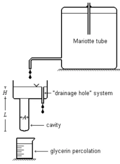
The device used for theK0experimental measurement ba-sically consists of a Mariotte tube and a ‘drainage hole’ sys-tem (Figure 1). The height of the ‘drainage hole’ imposes a constantHhydraulic load on the investigated empty cavities (Figure 2). This system can be coupled either to the cylinder or to the box. Experiments were carried out with glycerin with three different viscosity values.
The choice of the glycerin is because the Darcy’s law is not universally valid for all conditions of liquid flow in porous media. As the cavities are empties if water was used as per-colating fluid the flow velocity it would be very high. In this specific case the linearity of the flux versus hydraulic gradi-ent relationship fails. In the experimgradi-ent the Reynolds number (Re) was determined to guarantee the use of the Darcy’s law to evaluateK0(Re<1).
The cylinder and box have the following dimensions: 0.45 cm × 20.5 cm (diameter x length) and 0.635 cm ×
0.635 cm×4.7 cm (width×height×length).
The experimental procedure involved the following steps: 1) saturation of the empty cavities by glycerin; 2) glycerin viscosity measurement by the Stokes method; 3) glycerin viscosity measurement by the cylinder method [9]; 4) mea-surement of glycerin percolated through cavities to obtain its volume; 5) measurement of time interval for glycerin perco-lation; and 6) use of the Darcy’s law to calculate the saturated conductivityK0(cm s−1)of the empty cavity:
K0= V A t
L
(L+H) (1)
whereV(cm3)is the percolated glycerin volume,A(cm2) is the cross section area,t(s)the percolated volume time inter-val,L(cm)is the height andH(cm)is the glycerin column height above the cavity (Figure 1).
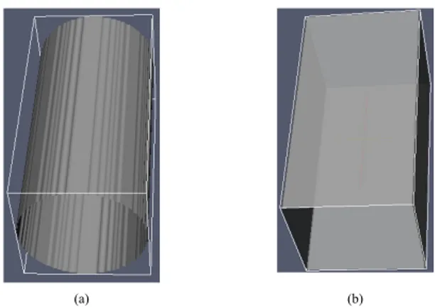
(a) (b)
FIG. 2: Empty cavities used for the evaluation ofK0(saturated con-ductivity). (a) cylinder and (b) box.
The measurements of cavitiesK0 and the glycerin kine-matic viscosityv(cm2s−1)occurred at the same temperature, which was monitored with the 0.1◦C resolution.
2.2. Analytical solutions
The cylinder and boxK0 is obtained by solving the NS equation for a Newtonian fluid in an incompressible regime and a non-slip condition on the walls [10,11]. TheK0 analyt-ical expression for ad diameter cylinder is well known and is presented in equation (2):
K0cylinder=
d2 32 g
v, (2)
in whichg(cm s−2)is the gravity acceleration.
For a box with a side square straight section area l(cm) the analytical expression forK0is given by [10]:
K0box=
l2 12
g
ν 1−6
∞
∑
n=1tanhαn
α5
n !
, (3)
in whichαn= (2n−1)π2, n=1,2, ....
2.3. Numerical simulation
ForK0values obtained through computational methods, the Boltzmann model was used. The three-dimensional physical space represented in the simulation, necessarily has to be discretized and a three-dimensional lattice is used for this. The sites in this lattice might represent solid and pores. Being a site in the lattice located by the vector~X and having bm neighbors, the evolution equation for the particle distri-bution functionNi(~X,T)is given by the so-called “Lattice Boltzmann Equation”:
Ni(~X+~ci,T+1) =Ni(~X,T) +Ωi(~X,T), (4) whereTis the time discrete variable,iis the direction of one of the closestbmneighbors,~cithe velocity vector in direction
i, withi=0 representing thebrresting particles.
The dynamics occurs in two steps in this model, the col-lision and the propagation steps. Colcol-lision is the step that simulates the molecular collisions needed so that thermody-namic equilibrium occurs; this step is represented by the term
Ωi(~X,T) in equation (4), called collision operator. At the collision step time is not incremented. This step is local and does not involve interactions with neighboring sites:
Ni′(~X,T) =Ni(X~,T) +Ωi(~X,T), (5) The variableNi′(~X,T)is called “collided” distribution func-tion and represents a new value at the same site~X and the same step of timeT.
Equation (4) represents the propagation step, it transports the collided termNi′(~X,T)to the neighboring site~X+~ci, at posterior timeT+1. A simple and sufficient form of colli-sion operator which recovers the NS macroscopic equation is known as BGK1[12] operator:
Ωi=
Nieq−Ni
τ , (6)
whereτis the relaxation time, which regulates the number of time steps that theNiparticle distribution takes to get closer to the equilibrium distributionNieq. That is, ifNi<Nieq,Ωi> 0 and the termΩi will be added to Ni making Ni tend to
Nieq, the same analysis might be done for the case in which Ni>Nieq.
The particle densityρin a site and the momentum, in this method are given by:
b
∑
i=0Ni=ρ, (7)
bm
∑
i=1Ni~ci=ρ~u. (8)
Taking that into consideration and imposing conservation of mass and momentum to the collision operator:
b
∑
i=0Ωi=0, (9)
bm
∑
i=1Ωi~ci=0, (10)
whereb=br+bm.
Particle distribution for theNieqis usually obtained through theNieqexpansion, in power series at the macroscopic veloc-ity~u, beingO(u2)sufficient so that NS equation is recov-ered. In this case, demands onNieq, besides conditions given by equations (7) and (8) are that the pressure be independent from macroscopic velocity and obey the flow density tensor of the momentum:
bm
∑
i=0Nieqciαciβ=pδαβ+ρuαuβ, (11)
whereciαis theαcomponent ofciand the hydrostatic pres-surepis given by:
p=bmc 2
bD ρ, (12)
whereDis the Euclidian dimension of space in which the lattice is immerse andc2=|ci|2. With this, the balance dis-tribution form for moving particles is given by:
Nieq=ρ
b+
ρD
bmc2
ciαuα+
ρD(D+2)
2bmc4
ciαuαciβuβ−
ρD
2bmc2
u2. (13) In the main directions x, y andz the equilibrium distri-bution must be doubled (Nieq =2Nieq) so that viscosity is isotropic [13].
Resting particles have the following equilibrium distribu-tion:
Noeq=ρ
bbr−
ρ
c2u
2. (14)
For a macroscopic analysis of the dynamics proposed by equation (4) timeδand space scaleshare usually used and the Knudsen variablekn=hL=Tδc is defined, whereLandTc are, respectively, the macroscopic characteristic length and time. With this, the Chapman-Enskog [14] method can be used, considering the equilibrium distribution disturbance, to
show that equation (4) becomes the Navier-Stokes, given by equation (15), disregarding the O(k2n) contributions:
∂t(ρuβ) +∂α(p)δαβ+∂α(ρuαuβ) =vρ∂α(∂αuβ+∂βuα), (15) in whichαandβare indexes that represent the spatial coor-dinatesx,yorz. For these indexes Einstein’s notation is seen (repeated indexes sum). The equation (15) is theβ compo-nent of the NS equation with kinematic viscosityvgiven by:
v= h 2c2
δ(D+2)
τ−1
2
. (16)
The boundary conditions used in the simulation are pe-riodic, that is, the fluid which leaves one end of the cavity is injected in the other end. The interaction between fluid and solid occurs so that there is no sliding, in this case, the ‘bounce back’ condition was adopted, in which a fluid parti-cle that collides with the walls has its velocity inverted. The program return permeabilityk, which is calculated (equation 17) with the Santos et al. [8] method, where in a stationary flow, the momentum applied to the fluid is equal to the loss of momentum on the walls:
k=vφ hmuxi hmuxilost
, (17)
in whichφis the porosity,hmuxiis the fluid average momen-tum in the cavity andhmuxilostis the average momentum lost by the fluid in the collisions with the cavity walls in a propa-gation step.
In order to obtainKfrom the permeability the relation be-low is used:
K=kg
v. (18)
3. RESULTS AND DISCUSSION
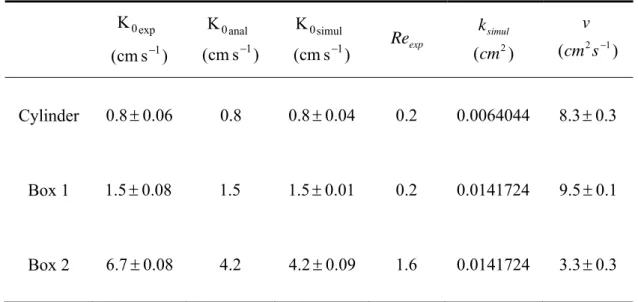
The experimental saturated conductivity values (K0exp), analytical (K0anal) and simulated (K0simul) for both empty cavities, as well as the simulated permeability (ksimul), are presented in table 1.
TheK0analvalue for the cylinder is found through equation (2), assumingd=0.45cm. The determination ofK0analfor the box is carried out through equation (3), consideringl= 0.635cm, where the two first terms in the infinite series are sufficient to obtain good approximation.
In simulations the necessity to represent cavities (Figure 2) through a discrete lattice, raises the need of evaluating a minimum value for the cavities dimensions in which the dis-cretization problems are minimized. The value of 200 sites for the lateral dimensionlof the box was chosen based on results of figure 3, where the permeability dependencekis shown, calculated in the simulation for a square box, accord-ing to the sidelof the box (for the cylinder, the same behav-ior is observed).
The scale factor used in simulations was h = 0.635 200 = 0.003175 for the box andh=0.45
TABLE 1: Saturated conductivity (K0) results for the three analyzed methods (analytical, experimental, and simulated). The value of gravity acceleration used in the calculations was 979 cm.s−2
)
s
cm
(
K
1 exp 0
−
)
s
cm
(
K
1 anal 0
−
)
s
cm
(
K
1 simul 0
−
Re
exp)
(
2cm
k
simul)
(
2 −1s
cm
v
Cylinder
0
.
8
±
0
.
06
0
.
8
0
.
8
±
0
.
04
0
.
2
0
.
0064044
8
.
3
±
0
.
3
Box 1
1
.
5
±
0
.
08
1
.
5
1
.
5
±
0
.
01
0
.
2
0
.
0141724
9
.
5
±
0
.
1
Box 2
6
.
7
±
0
.
08
4
.
2
4
.
2
±
0
.
09
1
.
6
0
.
0141724
3
.
3
±
0
.
3
Errors of K0 (experimental and simulated) and ν were obtained by error propagation.
1.41
1.42 1.43 1.44 1.45
0 25 50 75 100 125 150 175 200 l (site)
k (10
-2 cm 2 )
FIG. 3: Simulated permeability (k) values in function of the box width (l).
(a) (b) (c)
FIG. 4: Velocity fields for the cavities with different dimensions. Greater and darker arrows represent higher velocities. (a) Box with dimensions of 200 sites×200 sites×1 site; (b) and 40×40×40 and (c) cylinder with 200 diameter and 1 high.
A constant control of temperature was kept in the exper-iments aiming at minimizing the variations in theK0 mea-surement, since viscosity, which originated from molecules collision, suffers great variations with the temperature and strongly influences theK0results.
The Boltzmann model simulates the NS equation because its dynamics respects the mass conservation principles as well as the momentum, being such conditions fundamental
to the Newtonian fluid flow at a constant temperature. There-fore, simulations captured the physics relevant to the flow in the experimental arrangement of the tested cavities, present-ing excellent agreement with experimental results, validatpresent-ing the model.
Once flows of interest in the soil physics area are framed in the flow profile addressed by this work, water flow in soil samples usually occur with Re< 1 [15]. AsKexperimental measurements usually present difficulties, numeric simula-tion might be an interesting alternative for future predicsimula-tions of this physical property without the need to collect sam-ples and experimental measurements. This way, Boltzmann method appears as an alternative tool which might contribute with the development of this knowledge area in the future.
4. CONCLUSIONS
Results of this work lead to the following conclusions:
1. Fluid viscosity monitoring during K0 experimental measurements compensates possible errors due to tem-perature variations;
2. Results obtained show good agreement of the three methods of K0 measurement (analytical, experimen-tal, and simulated) when Re< 1. For box 2, whose Re> 1, percentage deviation between simulated (or analytical) and experimental was 59.5%;
3. Boltzmann model is a tool with potential for further work involving K0 measurements for more complex porous media.
Acknowledgements
Foundation and Capes for the master scholarship.
To Drs. Luiz Emerich dos Santos and Fabiano Gilberto Wolf of the Laboratory of Porous Media and Thermophysics
Properties (LMPT) of UFSC (Federal University of Santa Catarina) by the theoretical contributions.
[1] A. Klute, C. Dirksen, Hydraulic conductivity and diffusivity: Laboratory methods. In: BLACK, C.A. (Ed.) Methods of Soil Analysis. I. Physical and Mineralogical Methods. Madison, ASA/SSSA, 1986. pp.697-734.
[2] K. Reichardt, L.C. Timm, Solo, planta e atmosfera: conceitos, processos e aplicac¸˜oes. Barueri: Manole, 2004. 478p. [3] F.A.M. C´assaro, L.F. Pires, R.A. Santos, D. Gimenez, K.
Re-ichardt, Funil de Haines modificado: curvas de retenc¸˜ao de solos pr´oximos `a saturac¸˜ao. Revista Brasileira de Ciˆencia do Solo, 32:2555-2562, 2008.
[4] L. Alexander, R.W. Skaggs, Predicting unsaturated hydraulic conductivity from the water characteristic. Transactions of the ASAE, 29:176-184, 1986.
[5] M.C. Falleiros, O. Portezan, J.C.M. Oliveira, O.O.S. Bacchi, K. Reichardt, Spatial and temporal variability of soil hydraulic conductivity in relation to soil water distribution, using an ex-ponential model. Soil Technology, 45:279-285, 1998. [6] J. Zhuang, K. Nakayama, G.R. Yu, T. Miyazaki, Predicting
unsaturated hydraulic conductivity of soil based on some basic soil properties. Soil and Tillage Research, 59:143-154, 2001. [7] M.-E. Kutay, A.H. Aydilek, E. Masad, Laboratory validation
of lattice Boltzmann method for modeling pore-scale flow in granular materials. Computers and Geotechnics, 33:381–395, 2006.
[8] L.O.E. Santos, C.E.P. Ortiz, H.C. Gaspari, G.E. Haverroth, P.C. Philippi, Prediction Of Intrinsic Permeabilities With Lat-tice Boltzmann Method In: 18TH International Congress of Mechanical Engineering, 2005, Ouro Preto. Proceedings of COBEM 2005. Rio de Janeiro: ABCM, 2005. v. 1.
[9] P.L. Libardi, Dinˆamica da ´agua no solo. Piracicaba, 2004. P. L. Libardi, 2004. 420p.
[10] T.C. Papanastasiou, C.G. Georgios, N.A. Andreas, Viscous Fluid Flow. Boca Raton: CRC Press, 2000. 275 p.
[11] M.C. Potter, D.C. Wiggert, Mecˆanica dos Fluidos. S˜ao Paulo, Cengance Learning, 2009. 223p.
[12] Y.H. Qian, D. D’humieres, P. Lallemand, Lattice BGK Models for Navier-Stokes Equation. Europhysics Letters, 17:479-484, 1992.
[13] D.H. Rothman, S. Zaleski, Lattice-gas cellular automata: sim-ple models of comsim-plex hydrodynamics. United Kingdom: Cambridge University Press, 1997. 297p.
[14] P.C. Facin, Modelo de Boltzmann Baseado em Mediadores de Campo Para Fluidos Imisc´ıveis. Tese de Doutorado, Programa de P´os-Graduao em Engenharia Mecˆanica, Universidade Fed-eral de Santa Catarina, Florian´opolis, 2003.