The Influence of Temporal Migration in the
Synchronization of Populations
†V. MANICA∗ and J.A.L. SILVA
Received on November 28, 2013 / Accepted on February 4, 2015
ABSTRACT.A discrete metapopulation model with temporal dependent migration is proposed in order to study the stability of synchronized dynamics. During each time step, we assume that there are two processes involved in the population dynamics: local patch dynamics and migration process between the patches that compose the metapopulation. We obtain an analytical criterion that depends on the local patch dynamics (Lyapunov number) and on the whole migration process. The stability of synchronized dynamics depends on how individuals disperse among the patches.
Keywords:metapopulation, temporal migration, synchronization.
1 INTRODUCTION
The forms of dispersion in a metapopulation system (populations of single-species that live in fragments called patches) can induce the whole system to multiple behaviors [1, 3, 4, 7, 13]. An interesting behavior related to the dispersal process is the synchronized dynamics where the populations in all patches evolve with the same density [11]. Its importance lies in the fact that if the whole metapopulation is not synchronized and a local population is extinct, it can be recolonized by individuals that migrate from neighboring patches (“rescue effect”), favoring the population persistence [2]. A considerable number of populations that live in distinct regions tend to cycle in synchrony. A well-documented example is the Canadian lynxes that presents synchronized dynamics in its densities fluctuations due to weather conditions [2, 11]. Another example is the vole populations in Norway that synchronize due to dispersal processes and birds predation [8].
Systems of discrete equations are often used to model metapopulations [1, 4, 7, 13]. A metapop-ulation model with patches linked by migration and subjected to external perturbations was con-sidered in [1]. The model is a discrete-time system composed by single species where a constant
*Corresponding author: Vanderlei Manica – E-mail: [email protected] V. Manica thanks CAPES for supporting his PhD at UFRGS.
†The paper was presented at CMAC-CO 2013.
fraction disperses per generation. Through numerical simulations, it was shown that chaos can prevent global extinctions when coupling is weak. In [4] was obtained an analytical result for the stability of synchronized trajectories by considering a model with an arbitrary number of patches linked by dispersal. An analytical result examining a special case of density-dependent dispersal was obtained in [13], concluding that this mechanism reduces the stability regions of the syn-chronous dynamics. Nevertheless, density independent dispersal is observed in the dispersal of insects, while density-dependent dispersal is observed in such widely different invertebrates as locusts, snails and copepods [6]. In this paper, we present a metapopulation model similar to the ones described in [1, 4, 13]. The main difference is the assumption of temporal dependent migration. This assumption can be used in order to describe the movements of species that move to other areas in different periods due to weather conditions or dependence of foraging resources.
In Section 2 we present the metapopulation model with temporal dependent migration. In Sec-tion 3 we analyze the asymptotic local stability of synchronized trajectories and obtain a criterion to its stability based on the calculation of the transversal Lyapunov numbers. In Section 4 we present numerical simulations. Final comments and discussion are done in Section 5.
2 METAPOPULATION MODEL
The metapopulation model consists ofd equal patches labeled as 1,2, . . . ,d. We assume that the processes of survival and reproduction which compose the local dynamics is described by a map f on[0,∞)of classC1. In the absence of dispersal between patches, the time evolution of the population is given by
xt+1= f(xt), t =0,1,2, . . . , (2.1)
wherext represents the number of individuals at timet.
We assume that a fraction of individuals leaves patchiand disperses to the neighboring patches. We assume that the migration fraction is temporal dependent, that is, it is given by a map on [0,1] such thatmt+1 = g(mt), where mt is the migration fraction at timet. Thus, the density of individuals that leaves patchi is given bymtf(xti), wherexti denotes the population density in patchi at timet, for alli =1, . . . ,d,t =0,1, . . .. Moreover, from individuals that disperse from neighboring patchesk, a fractionγikreaches patchi. The dispersal fractions of individuals that migrate among the patches is described by a nonnegative matrixŴwith entriesγik,i,k = 1,2, . . . ,d. Eachγik represents the fraction of individuals coming from patchkthat will settle in patchi (Fig. 1). We assume that there is no loss of individuals and the individuals do not return to the original patch, therefored
i=1 γik =1 andγkk =0 for allk =1, . . . ,d. Taking these into consideration, we can write a system of equations describing the dynamics of the metapopulation by
xit+1=(1−mt)f(xti)+ d
k=1
The first term in equation (2.2) represents the individuals that did not leave patchi at timet, while the second term is the sum of all contributions of individuals from neighboring patches.
Figure 1: Schematic represetation of the migration process. After patch local dynamics, a frac-tion of individualsmt leaves patchkat time stept. From these individuals a fractionγik moves to patchi. Thus, the fraction of individuals that leaves patchkand reaches patckiismtγik.
3 SYNCHRONIZATION AND TRANSVERSAL STABILITY
We assume that synchronization is achieved if the population density of all patches is the same, that is, xti = xts, for alli = 1,2, . . . ,d andt = 0,1,2, . . .. Synchronized solutions of the system (2.2) may not exist if the system lacks some symmetry. Substitution of xti = xts in equation (2.2) leads us to the existence of such synchronized solution provided d
k=1γik = 1,i =1,2, . . . ,d. Furthermore, the dynamics of each patch in the synchronized state satisfies xs
t+1= f(xst)which is equivalent to equation (2.1), the single patch model equation. In other words the metapopulation synchronizes with the same dynamics of a single isolated patch.
We are interested in studying the local asymptotic stability of the synchronized state, that is, whether orbits that initiate close to the synchronized state will be attracted to it. In order to achieve this goal, we linearize the equation (2.2) around the synchronized trajectory, obtaining
t+1=J(xst)t, (3.3)
wheret ∈Rdis the perturbation of the synchronized trajectory, andJ(xst)is thed×dJacobian matrix of system (2.2) evaluated at xst, wherexst = (xst,xst, . . . ,xst) ∈ Rd. Notice that the Jacobian matrixJ(xst)has its entries given by
αik =
(1−mt)f ′
(xts), ifi =k;
γikmtf ′
(xts), ifi =k.
Thus, it can be written as
J(xst)=(I−mtB)f ′
(xts), (3.4)
whereI is the identity matrix andB=I −Ŵ.
It is important to notice that the connectivity matrixŴis doubly stochastic (all rows and columns add up to one). An application of the Perron-Frobenius Theorem [9] leads to the fact thatλ0= 1 is the dominant eigenvalue ofŴ. Moreover, its eigenspace is spanned by the vector 1 = [1 1 . . . 1]T ∈ Rd which correspond to the in-phase state, that is, the diagonal of the phase space
We assume thatŴis diagonalizable which allows us to express the Jacobian matrix as a diagonal matrix and the local stability of the synchronized state can be analyzed through the diagonal terms. With this assumption, there exists an invertible matrixQsuch that
Ŵ=Qdiag(1, λ1, . . . , λd−1)Q−1.
It allows us to write the Jacobian matrix (3.4) in the following diagonal form
J(xst)=Q ⎛
⎜ ⎜ ⎜ ⎜ ⎜ ⎝
1 0 . . . 0
0 1−mt +λ1mt . .. ... ..
. . .. . .. 0
0 . . . 0 1−mt +λd−1mt
⎞
⎟ ⎟ ⎟ ⎟ ⎟ ⎠
f′(xst)Q−1. (3.5)
Thus, the synchronized state will be stable if transversal perturbations to the synchronized state shrink to zero. To reach this goal, we define the maximum transversal Lyapunov number,K, by
K(x0s,m0)= max
i=1,...,d−1τlim→∞ Pτ−1,i·. . .·P1,iP0,i
1/τ,
(3.6)
wherePt,i = f ′
(xts)(1−mt+λimt). Consequently, the transversal perturbation tends to zero if K(x0s,m0) <1.
Observe that
|Pτ−1,i·. . .·P0,i|
=
τ−1
t=0
|f′(xst)|
|(1−mτ−1+λimτ−1)·. . .·(1−m0+λim0)|,
(3.7)
thus, we can write the maximum transversal Lyapunov number as
K(xs0,m0)=L(x0s)(m0), (3.8)
where
L(x0s)= lim
τ→∞ (
τ−1
t=0
|f′(xst)|)1/τ (3.9)
is the Lyapunov number of f starting atx0s and
(m0)= max
i=1,2,...,d−1 τlim→∞ (|(1−mτ−1+λimτ−1)·. . .·(1−m0+λim0)|)
1/τ (3.10)
is a quantifier that depends on the initial migration rate.
and state a criterion for the local asymptotic stability of an attractor in the synchronized invariant state given by
K=L <1, (3.11)
where
L =exp
∞
0
ln|f′(x)|dρ(x)
. (3.12)
and
= max
i=1,...,d−1 exp [0,1]ln|1−mλi |
dρ(m). (3.13)
Notice thatL depends on the patch local dynamics whiledepends on the whole migratory process. It is important to observe that the evolution of the term that corresponds to the value 1 in the Jacobian matrix (3.5) is exactly the Lyapunov number and it gives the behavior of the synchronized trajectory within the phase space diagonal, that is, a periodic trajectory (L <1) or a chaotic trajectory (L >1).
In the following, we calculate the quantifier given in (3.13) to different temporal migration rules. In subsection 3.1 we assume that the mapgthat generates the temporal migration fractions has a stable cycle and a periodic behaviour. In subsection 3.2 we assume the temporal migration rates are given by a uniform distribution.
3.1 Temporal migration given by a Dirac measure
A Dirac measure is a measureδydefined on a setEsuch that
δy =
1, y∈ E;
0, c.c.. (3.14)
Letδm0 denote the Dirac measure centered on the fixed migration ratem0. Thus, we have
= max
i=1,...,d−1 exp [0,1]ln|1−mλi |dδm0
= max
i=1,...,d−1 exp(ln|1−m0λi |)
= max
i=1,...,d−1(|1−m0λi |).
(3.15)
In this case, the criterion established in (3.11) is the same established by Earn et al. [4] that considered a metapopulation with any number of patches arbitrarily connected.
If we assume that the probability measure is concentrated in two periodic points,m0andm1, we have
= max
i=1,...,d−1 exp [0,1]
ln|1−mλi |dδm0,m1
= max
i=1,...,d−1 exp
ln|1−m0λi | +ln|1−m1λi | 2
= max
i=1,...,d−1exp(ln(|1−m0λi | · |1−m1λi |)
1
2)
= max
i=1,...,d−1(|1−m0λi | · |1−m1λi |)
1
2.
In this case, the quantifieris the geometric average of(1−m0λi)and(1−m1λi). In fact, if the migration rates are distributed inpperiodic points,m0,m1, . . . ,mp−1, the quantifieris
given by the following geometric average
= max i=1,...,d−1
|1−m0λi | ·. . .· |1−mp−1λi | 1
p. (3.17)
3.2 Temporal migration given by a uniform distribution
Now we assume that the temporal migration rates are given by a uniform distribution. In our case, the probability density function with a uniform distribution on a set[a,b] ⊂ [0,1]is
p(m)= ⎧ ⎪ ⎪ ⎨ ⎪ ⎪ ⎩
p1=0, 0≤m<a;
p2= b−1a, a≤m<b;
p3=0, b≤m<1.
(3.18)
Observe thatρ(m)=1
0 p(m)dm =
b a
1
b−adm=1. Besides that, we can write (3.13) as
= max i=1,...,d−1 exp
1
b−a
[a,b]ln
|1−mλi |dm
. (3.19)
The above integral can be solved analytically resulting
= ⎧ ⎪ ⎪ ⎪ ⎪ ⎨ ⎪ ⎪ ⎪ ⎪ ⎩ max i=1,...,d−1
1 e
(1−aλ
i)(1−aλi) (1−bλi)(1−bλi)
λ 1 i(b−a)
, if 0≤m<λi1;
max i=1,...,d−1
1 e
(bλ
i−1)(bλi−1) (aλi−1)(aλi−1)
λ 1 i(b−a)
, if λ1
i ≤m≤1.
(3.20)
In the following, we perform numerical simulations to illustrate the stability regions of synchro-nized solutions and present the values of the quantifierto different temporal migration rules.
4 NUMERICAL SIMULATIONS
We perform numerical simulation to illustrate the behavior of our network of patches connected by temporal dependent migration. In order to determine whether synchronization occurs we define the synchronization error,et, by
et = 1 d
d
i=1
xti−xti+1
(4.21)
wherextd+1=xt1. Synchronization is detected whenet →0.
We consider that the local dynamics is given by the following Ricker function
wherex represents the patch density andr is the intrinsic growth rate (r >0). The dynamics of a local habitat with the Ricker model is well-known and exhibits equilibrium, periodic and chaotic dynamics depending on the growth rate [10]. For 0<r <2, the local dynamics become a state of equilibrium. For 2<r <2.526, the equilibrium point is unstable and a two-periodic trajectory takes its place. Asris increased, there appears a four-periodic trajectory and the two-periodic become unstable and we can observe period doubling bifurcations to chaos. In order to simulate chaotic within patch dynamics we assumer =3.1, which implies that the isolated patch model has a chaotic trajectory with Lyapunov numberL ≈1.327.
The configuration matrixŴcan be defined in different forms. Two well-known configurations are the nearest neighbor coupling and the global coupling [4]. We illustrate our results considering the patches linked in a ring format with the two-nearest neighbors coupling, whose configuration matrix,Ŵ, is given by
Ŵ=
⎛
⎜ ⎜ ⎜ ⎜ ⎜ ⎜ ⎜ ⎜ ⎜ ⎝
0 1/2 0 . . . 0 1/2 1/2 0 1/2 0 . . . 0
0 1/2 . .. . .. . .. ... ..
. . .. . .. 0 1/2 0 0 . . . 0 1/2 0 1/2 1/2 0 . . . 0 1/2 0
⎞
⎟ ⎟ ⎟ ⎟ ⎟ ⎟ ⎟ ⎟ ⎟ ⎠
. (4.23)
In this case, the eigenvalues ofŴare given byλ0=1 andλi =cos2dπi,i =1,2, . . . ,d−1. Of course, other local patch dynamics and configuration network topologies could be used, but our main concernment is to show the different behavior generated by temporal migration rates.
Figure 2 shows the bifurcation diagram of the synchronization error and the respective maximum transversal Lyapunov number versus the migration rate. In all cases, individuals migrate with the same rate at timet. We can observe that the non-synchronization region is characterized by weak interaction. Moreover, the increase in the number of patches decreases the synchronization region and increase the maximum transversal Lyapunov number. In fact, the subdominant eigenvalue of the matrixŴtends to one as n → +∞(λi → 1 asd → +∞,i = 1,2, . . . ,d−1), thus the quantifiergiven in (3.15) also tends to one asd → +∞ (see [12]). It means that the stability criterion will approach to the Lyapunov number if we increase the number of patches. Moreover, the synchronized attractors will be unstable for any value of the migration rate if the local dynamics of a single isolated patch is chaotic (L>1).
0 0.5 1 0 1 2 3 m et
(a)
0 0.5 1
0 1 2 3 m e t
(b)
0 0.5 1
0 1 2 3 m e t (c)
0 0.5 1
0 0.5 1 1.5 m K Λ (d)
0 0.5 1
0 0.5 1 1.5 m K Λ (e)
0 0.5 1
0 0.5 1 1.5 m K Λ (f)
Figure 2: Synchronization error ((a), (b) and (c)) and respectably maximum transversal Lya-punov number ((d), (e) and (f)) vs m. Local dynamics is given by the Ricker function f(x) = xexp(r(1 −x))withr = 3.1. The patches are coupled with the two-nearest neigh-bors coupling. (a) 2 patches. (b) 5 patches. (c) 10 patches.
0 0.5 1
0 0.5 1 1.5 m K Λ (d)
0 0.5 1
0 1 2 3 m e t
(a)
0 0.5 1
0 1 2 3 m e t
(b)
0 0.5 1
0 0.5 1 1.5 m K Λ (e)
0 0.5 1
0 0.5 1 1.5 m K Λ (f)
0 0.5 1
0 1 2 3 m e t (c)
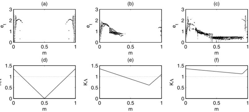
Figure 3: Synchronization error ((a), (b) and (c)) and respective maximum Lyapunov number ((d), (e) and (f))vs m. Local dynamics is given by the Ricker function f(x)=xexp(r(1−x)) withr = 3.1. Five patches are coupled with the two-nearest neighbors. (a)m0 = m and m1=0.1. (b)m0=mandm1=0.5. (c)m0=mandm1=0.9.
Table 1: Quantifierfor different temporal migration rates. Temporal migration rates are distributed aroundm=0.3. We can observe that the values ofdo not change significantly.
Fixed Point Period 2 Period 4 Uniform Uniform
m 0.3 0.2 and 0.4 0.15, 0.25, 0.35 and 0.45 [0.2, 0.4] [0.1, 0.5]
0.7927 0.78968 0.78892 0.7916 0.7887
5 DISCUSSION
In this paper we develop a model of a network of equal patches linked by temporal dependent migration. The time evolution of the system involves two processes: local patch dynamics and migration between the patches. We then analyze the phenomenon of synchronization between the patches. We obtain an analytical criterion for the local asymptotic stability of synchronized trajectories based on the computation of the transversal Lyapunov numbers of attractors on the synchronous invariant manifold. The criterion is obtained via linearization process around the synchronized trajectories. The criterion is given by the product of two quantifiers: the separation rate of two nearby orbits in the single isolated patch measured by the Lyapunov number,L, and a quantifier that depends on the whole migration process,(eq. 3.11 ). We then calculate the value of this quantifier to different migration rules. At first, we describeassuming the migration rate with a periodic behavior (eq. 3.17), we then consider the migration rate uniform distributed on the interval[a,b] ⊆ [0,1](eq. 3.20). The quantifier in the case of migration rates with a periodic behavior involves the migration rates and the eigenvalues of the matrix that inform the network topology between the patches, while in the case of uniform distribution also involves the size of the interval.
Our observation based on theoretical results and on numerical simulations reveals the impor-tance of analyzing a metapopulation model with temporal migration. We performed numerical simulation assuming each patch dynamics given by Ricker map with chaotic behavior. Then, we analyze the influence that the migration process has over synchronized dynamics. We observe that an increase in the number of patches decrease the stability regions (Fig. 2). Besides that, weak interactions between patches, decreases the size of stability regions, while intermediate and high migration rates have an opposite effect (Fig. 3). We observe that, if the temporal migra-tion rates are distributed around an average, the values of quantifierdo not change significantly (Table 1).
RESUMO.Um modelo metapopulacional com migrac¸˜ao dependente do tempo ´e proposto a fim de estudarmos a estabilidade de trajet´orias sincronizadas. Durante cada gerac¸˜ao, consi-deramos que existem dois processos na dinˆamica populacional: a dinˆamica local e a migra-c¸˜ao entre os s´ıtios que comp˜oem a metapopulamigra-c¸˜ao. Obtemos um crit´erio para a ocorrˆencia de sincronizac¸˜ao que depende da dinˆamica local (n´umero de Lyapunov) e de todo o processo migrat´orio. A estabilidade de trajet´orias sincronizadas depende de como os indiv´ıduos migram entre os s´ıtios.
REFERENCES
[1] J.C. Allen, W.M. Schauffer & D. Rosko. Chaos reduces species extinction by amplifying local popu-lation noise.Nature,364(1993), 229–232.
[2] B. Blasius, A. Huppert & L. Stone. Complex dynamics and phase synchronization in saptially ex-tended ecological systems.Nature,399(1999), 353–359.
[3] M. Doebeli. Dispersal and Dynamics.Theor. Pop. Biol.,47(1995), 82–106.
[4] D.J., Earn, S.A. Levin & P. Rohani. Coherence and Conservation.Science,290(2000), 1360–1364.
[5] J.P. Eckmann & D. Ruelle. Ergodic Theory of chaos and strange attractors. Rev. Modern Phys.,
57(1985), 617–656.
[6] L. Hansson. Dispersal and connectivity in metapopulations.Biol. J. Linn. Soc.,42(1991), 89–103.
[7] M. Heino, V. Kaitala, E. Ranta & J. Lindstr¨om. Synchronous dynamics and rates of extinction in spatially structured populations.Proc. R. Soc. London B,264(1997), 481–486.
[8] R.A. Ims & H.P. Andreassen. Spatial synchronization of vole population dynamics by predatory birds. Nature,408(2000), 194–196.
[9] P. Lancaster & M. Tismenetsky. The Theory of Matrices, Academic Press, London (1985).
[10] R.M. May. Biological populations with nonoverlapping generations: stable points, stable cycles, and chaos.Science,186(1974), 645–647.
[11] R.M. May & A.L. Lloyd. Synchronicity, chaos and population cycles: spatial coherence in an uncer-tain world.Trends Ecol. Evol.,14(1999), 417–418.
[12] J.A.L. Silva, M.L. De Castro & D.A.R. Justo. Synchronism in a metapopulation model.Bull. Math. Biol.,62(2000), 337–349.