Classical technical analysis of Latin American market indices.
Correlations in Latin American currencies (
ARS
,
CLP
,
M X P
)
exchange rates with respect to
DEM
,
GBP
,
J P Y
and
U SD
∗ †
M. Ausloos
1and K. Ivanova
2 1SUPRATECS, B5, Sart Tilman, B-4000 Li`ege, Euroland2Pennsylvania State University, University Park, PA 16802, USA
Received on 5 May, 2003
The classical technical analysis methods of financial time series based on the moving average and momentum is recalled. Illustrations use the IBM share price and Latin American (Argentinian MerVal, Brazilian Bovespa and Mexican IPC) market indices. We have also searched for scaling ranges and exponents in exchange rates between Latin American currencies (ARS,CLP,M XP) and other major currenciesDEM,GBP,JP Y,
U SD, andSDRs. We have sorted out correlations and anticorrelations of such exchange rates with respect to
DEM,GBP,JP Y andU SD. They indicate a very complex or speculative behavior.
1
Introduction
The buoyancy of the US dollar is a reproach to stagnant Japan, recessing Europe economy and troubled developing countries like Brazil or Argentina. Econophysics aims at introducing statistical physics techniques and physics mod-els in order to improve the understanding of financial and economic matters. Thus when this understanding is estab-lished, econophysics mightlaterhelp in the well being of humanity. In so doing several techniques have been devel-oped to analyze the correlations of the fluctuations of stocks or currency exchange rates. It is of interest to examine cases pertaining to rich or developing economies.
In the first sections of this report we recall the classical technical analysis methods of stock evolution. We recall the notion of moving averages and (classical) momentum. The case of IBM and Latin American market indices serve as illustrations.
In 1969 the International Monetary Fund created the special drawing rightsSDR, an artificial currency defined as a basket of national currencies DEM, F RF, U SD, GBP andJP Y. TheSDRis used as an international re-serve asset, to supplement members existing rere-serve assets (official holdings of gold, foreign exchange, and reserve po-sitions in the IMF). TheSDRis the IMF’s unit of account. Four countries maintain a currency peg against theSDR. Some private financial instruments are also denominated in SDRs.[1, 2] Because of the close connections between the developing countries and the IMF, we search for correla-tions between the fluctuacorrela-tions ofARS, CLP andM XP exchange rates with respect toSDRand the currencies that form this artificial money. In the latest sections of this re-port, we compare the correlations of such fluctuations as we
did in our previous results onEU Rexchange rates fluctua-tions with respect toU SD,GBP andJP Y [3, 4, 5].
2
Technical Analysis: IBM and Latin
America Markets
Technical indicators as moving average and momentum are part of the classical technical analysis and much used in efforts to predict market movements [6]. One question is whether these techniques provide adequate ways to read the trends.
Consider a time seriesx(t)given at N discrete timest. The series (or signal) moving average Mτ(t) over a time
intervalτis defined as Mτ(t) =
1
τ
t+τ−1
i=t
x(i−τ) t=τ+ 1, . . . , N (1) i.e. the average of xover the last τ data points. One can easily show that if the signalx(t)increases (decreases) with time, Mτ(t) < x(t)(Mτ(t) > x(t)). Thus, the moving
average captures the trend of the signal given the period of timeτ. The IBM daily closing value price signal between Jan 01, 1990 and Dec 31, 2000 is shown in Fig. 1 (top figure) together with Yahoo moving average taken forτ = 50days [7]. The bottom figure shows the dailyvolumein millions.
There can be as many trends as moving averages asτ intervals. The shorter theτ interval the more sensitive the moving average. However, a too short moving average may give false messages about the long time trend of the signal. In Fig. 2(a) two moving averages of the IBM signal forτ=5 days (i.e. 1 week) and 21 days (i.e. 1 month) are compared for illustration.
∗Happy Birthday, Dietrich; by now you should be rich !
†Note of the Editor: Due to a mistake, this article has not been published in the special issue of the Braz. J. Phys. (Volume33, number 3, 2003) dedicated
1990 1992 1994 1996 1998 2000 101
102
Price
IBM 50−day MA
19900 1992 1994 1996 1998 2000
20 40 60 80
Millions
Volume of Transactions
Figure 1. IBM daily closing value signal between Jan 01, 1990 and Dec 31, 2000, i.e. 2780 data points with Yahoo moving average for∆T
= 50 day. (top); the bottom figure shows the daily volume
1993.2 1993.4 1993.6 1993.8 1994 10
11 12 13 14 15 16
date
resistance death X
support gold X
IBM M5 M21
1990 1992 1994 1996 1998 2000
−4 −2 0 2 4 6 8 10 12
IBM Momentum
1 week 1 month 1 year
1999 2000 2001
−5 0 5
1990 1992 1994 1996 1998 2000
−20 0 20 40 60 80 100
IBM Σ Momentum
1 week 1 month 1 year
1999 2000 2001
−40 −20 0 20 40 60
12 1999 2 3 4 5 6 7 8 9 10 11 12 2000
−40 −20 0 20 40 60 80 100 120 140
Momentum indicators Moving averages
IBM Momentum
(2)
(3)
(5)
(1)
(4)
IBM week month year
Figure 2: (a) IBM daily closing value signal between Jan 01, 1990 and Dec 31, 2000, with two moving averages, Mτ1 and Mτ2 for
τ1 = 5days andτ2 = 21days. (b) IBM classical momentum (c) moving average of IBM classical momentum for three different time
The intersections of the price signal with a moving av-erage can define so-called lines of resistance or support [6]. A line of resistance is observed when the local maximum of the price signalx(t)crosses a moving averageMτ(t). A
support line is defined if the local minimum ofx(t)crosses Mτ(t). In Fig. 2(a) lines of resistance happen around May
1993 and lines of support around Sept 1993. Support levels indicate the price where the majority of investors believe that prices will move higher, and resistance levels indicate the price at which a majority of investors feel prices will move lower. Other features of the trends are the intersections be-tweentwomoving averagesMτ1andMτ2which are usually
due to drastic changes in the trend ofx(t)[8]. Consider two moving averages of IBM price signal forτ1 = 5days and τ2= 21days (Fig. 2(a)). Ifx(t)increases for a long period of time before decreasing rapidly,Mτ1will crossMτ2from
above. This event is called a ”death cross” in empirical fi-nance [6]. In contrast, whenMτ1crossesMτ2 from below,
the crossing point coincide with an upsurge of the signal x(t). This event is called a ”gold cross”. Therefore, it is of interest to study the density of crossing points between two moving averages as a function of the size difference of the τ’s defining the moving averages. Based on this idea, a new and efficient approach has been suggested in Ref.[8] in order to estimate an exponent that characterizes the roughness of a signal.
The so calledmomentumis another instrument of the technical analysis and we will refer to it here as the clas-sical momentum, in contrast to the generalized momentum [9]. The classical momentum of a stock is defined over a time intervalτas
Rτ(t) =
x(t)−x(t−τ)
τ =
∆x
∆t t=τ+ 1, . . . , N (2) The momentumRτ for three time intervals,τ = 5,21
and 250 days, i.e. one week, one month and one year, are shown in Fig. 2(b) for IBM. The longer the period the smoother the momentum signal. Much information on the price trend turns is usually considered to be found in a mov-ing average of the momentum
RΣ
τ(t) = t+τ−1
i=t
x(i)−x(i−τ)
τ t=τ+1, . . . , N (3) Moving averages of the classical momentum over 1 week, 1 month and 1 year for the IBM price differenceover the same time intervals,RΣ
τ are shown in Fig. 2(c). In Fig.
2(d) the IBM signal and its weekly (short-term), monthly (medium-term) and yearly (long-term) moving averages are compared to the weekly (short-term), monthly (medium-term) and yearly (long-(medium-term) momentum indicators in order to better observe the bullish and bearish trends in 1999.
The message that is coming out of reading the combina-tion of the these six indicators states that one could start buy-ing at the momentum bottom, as it is for both monthly and weekly momentum indicators around mid February 1999 and buy the rest of the position when the price confirms the momentum uptrend and rises above the monthly moving av-erage which is around March 1999. The first selling signal is
given during the second half of July 1999 by the death cross between short and medium term moving averages and by the maximum of the monthly momentum, which indicates the start of a selling. At the beginning of October 1999, occurs the maximum of the long-term momentum. It is rec-ommended that one can sell the rest of the position since the price is falling down below the moving average. Hence, it is said thatmomentum indicators lead the price trend. They give signals before the price trend turns over.
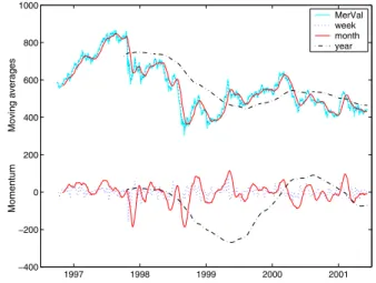
Along the lines of the above for IBM, we analyze three Latin America financial indices, Argentinian MerVal, Brazilian Bovespa and Mexican IPC (Indice de Precios y Cotizaciones) applying the moving averages and the classi-cal momentum concepts. In Fig. 3 the time evolution of the MerVal stock over the time interval mid 1996 - mid 2001, is plotted with a simple moving average forτ=50 days show-ing the medium range trend of the price. The movshow-ing aver-age and classical momentum of the MerVal stock prices for time horizons equal to one week, one month and one year are shown Fig. 3.
1997 1998 1999 2000 2001 −400
−200 0 200 400 600 800 1000
Momentum Moving averages
MerVal week month year
Figure 3. Argentinian MerVal daily closing value signal between Oct 08, 1996 and Jun 06, 2001, i.e. 1162 data points; classical mo-mentum for three time horizons, short-term (weekly) (dot curve), medium-term (monthly) (solid curve) and log-term (yearly) (dot-dash curve).
The cases of the Brazilian Bovespa and Mexican IPC (Indice de Precios y Cotizaciones) are shown in Figs. 4 and 5 respectively.
3
Exchange Rates and Special
Draw-ing Rights
SDRs. TheSDRserves as the unit of account for a num-ber of other international organizations, including the WB. Four countries maintain a currency peg against the SDR. Some private financial instruments are also denominated in SDRs.
1994 1996 1998 2000 −5000
0 5000 10000 15000 20000
Momentum Moving averages
Bovespa week month year
Figure 4. Brazilian Bovespa daily closing value signal between April 27, 1993 and Jun 06, 2001, i.e. 2010 data points; classi-cal momentum for three time horizons, short-term (weekly) (dot curve), medium-term (monthly) (solid curve) and log-term (yearly) (dot-dash curve).
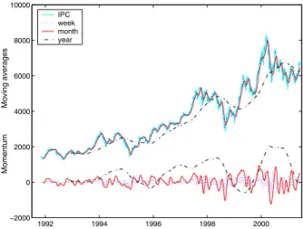
1992 1994 1996 1998 2000 −2000
0 2000 4000 6000 8000 10000
Momentum Moving averages
IPC week month year
Figure 5. Mexican IPC daily closing value signal between Nov. 08, 1991 and Jun 06, 2001, i.e. 2384 data points; classical mo-mentum for three time horizons, short-term (weekly) (dot curve), medium-term (monthly) (solid curve) and log-term (yearly) (dot-dash curve).
The basket is reviewed every five years to ensure that the currencies included in the basket are representative of those used in international transactions and that the weights assigned to the currencies reflect their relative importance in the world’s trading and financial systems. Following the completion of the most recent regular review ofSDR valua-tion on October 11, 2000, the IMF’s Executive Board agreed on changes in the method of valuation of theSDRand the determination of theSDRinterest rate, effective Jan. 01, 2001.
The SDR artificial currency can be represented as an weighted sum of the five currenciesCi,i= 1,5:
1SDR=
5
i=1
γiCi (4)
whereγiare the currencies weights in percentage (Table 1)
andCidenote the respective currencies, U.S. Dollar (U SD),
German Mark (DEM), French Franc (F RF), Japanese Yen (JP Y), British Pound (GBP).
Table 1: Currency Weights inSDRBasket (In Percent) Currency Last Revision Revision of
January 1, 2001 January 1, 1996
U SD 45 39
EU R 29
DEM 21
F RF 11
JP Y 15 18
GBP 11 11
On January 1, 1999, the German Mark and French Franc in theSDRbasket were replaced by equivalent amounts of EU R. The relevant exchange rates (ExR) are shown in Figs. 6-8.
3.1
The DFA technique
The DFA technique [10] is often used to study the correla-tions in the fluctuacorrela-tions of stochastic time series like the cur-rency exchange rates. Recall briefly that the DFA technique consists in dividing a time seriesy(t)of lengthN intoN/τ nonoverlapping boxes (called also windows), each contain-ingτ points [10]. The local trendz(n)in each box is de-fined to be the ordinate of a linear least-square fit of the data points in that box. The detrended fluctuation functionF2(τ) is then calculated following:
⌋
F2(τ) = 1
τ (k+1)τ
n=kτ+1
[y(n)−z(n)]2 k= 0,1,2, . . . ,
N τ −1
(5)
1997 1998 1999 2000 2001 1.25
1.3 1.35 1.4 1.45 1.5
ARS/SDR
1997 1998 1999 2000 2001 0.99
0.995 1
ARS/USD
1997 1998 1999 2000 2001 0.4
0.45 0.5 0.55 0.6 0.65 0.7 0.75
ARS/DEM
1997 1998 1999 2000 2001 6.5
7 7.5 8 8.5 9 9.5 10x 10
−3
ARS/JPY
1997 1998 1999 2000 2001 1.35
1.4 1.45 1.5 1.55 1.6 1.65 1.7 1.75
ARS/GBP
Figure 6. Exchange rates ofARSwith respect toSDR,U SD,DEM,JP Y,GBPfor the time interval between Aug. 6, 1996 and May 31, 2001, i.e. 1208 data points, as available on http://pacific.commerce.ubc.ca/xr/ website .
1997 1998 1999 2000 2001 550
600 650 700 750 800
CLP/SDR
1997 1998 1999 2000 2001 400
450 500 550 600 650
CLP/USD
1997 1998 1999 2000 2001 220
230 240 250 260 270 280 290 300 310
CLP/DEM
1997 1998 1999 2000 2001 3
3.5 4 4.5 5 5.5
CLP/JPY
1997 1998 1999 2000 2001 600
650 700 750 800 850 900 950
CLP/GBP
1997 1998 1999 2000 2001 10
10.5 11 11.5 12 12.5 13 13.5 14 14.5 15
MXP/SDR
1997 1998 1999 2000 2001 7
7.5 8 8.5 9 9.5 10 10.5 11
MXP/USD
1997 1998 1999 2000 2001 3.5
4 4.5 5 5.5 6 6.5
MXP/DEM
1997 1998 1999 2000 2001 0.06
0.065 0.07 0.075 0.08 0.085 0.09 0.095 0.1 0.105
MXP/JPY
1997 1998 1999 2000 2001 11
12 13 14 15 16 17 18
MXP/GBP
Figure 8. Exchange rates ofM XP with respect toSDR,U SD,DEM,JP Y,GBPfor the time interval between July 7, 1993 and May 31, 2001, i.e. 1975 data points, as available on http://pacific.commerce.ubc.ca/xr/ website.
AveragingF2(τ)over theN/τintervals gives the mean-square fluctuations
φ(τ) =< F2(τ)>1/2∼τα (6) The exponent αvalue implies the existence or not of long-range correlations, and is assumed to be identical to the Hurst exponent when the data is stationary. Moreover,αis an accurate measure of the most characteristic (maximum) dimension of a multifractal process [11]. Since only the
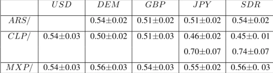
slopes and scaling ranges are of interest the various DFA-functionsφ(τ)have been arbitrarily displaced for readabil-ity in Figs. 9-11. Theα values are summarized in Table 2. It can be noted that the scaling ranges are usually from 5 days till 170 days forARSexchange rates, from 5 days to about 1 year forM XP andCLP exchange rates, with the exponentαclose to 0.5 in that range. Crossover at 80 days from Brownian like to persistent correlations is obtained for CLP/JP Y andCLP/SDR.
Table 2.αexponent for the scaling regime of considered ExR in the text
U SD DEM GBP JP Y SDR
ARS/ 0.54±0.02 0.51±0.02 0.51±0.02 0.54±0.02 CLP/ 0.54±0.03 0.50±0.02 0.51±0.03 0.46±0.02 0.45±0. 01 0.70±0.07 0.74±0.07 M XP/ 0.54±0.03 0.56±0.03 0.54±0.03 0.55±0.02 0.56±0. 03
3.2
Local scaling with DFA and
Intercorrela-tions between fluctuaIntercorrela-tions
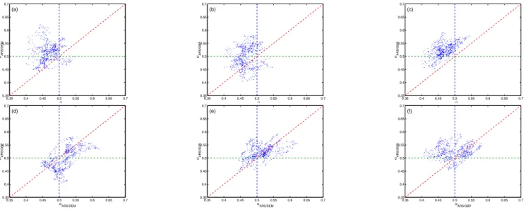
The time derivative of α can usually be correlated to an entropy production [12] through market information ex-changes. As done elsewhere, in order to probe the existence oflocally correlatedanddecorrelatedsequences, we have constructed an observation box, i.e. a 500 days wide win-dow probe placed at the beginning of the data, calculatedα for the data in that box. Moving this box by one day toward the right along the signal sequence and again calculatingα, a localαexponent is found (but not displayed here).
We eliminate the time between these data sets and con-struct a graphical correlation matrix of the time-dependentα exponents for the various exchange rates of interest (Fig.12-14). We showαCi/Bj vs. another αCi/Bj, where aCi is
a developing country currency while Bj is U SD, GBP,
100 101 102 103 10−5
10−4 10−3 10−2 10−1
t(days)
<F
2 (t)>
1/2
JPY DEM SDR GBP ARS /
Figure 9. DFA-functionφ(τ)function for theARSExchange rates shown in Fig. 6; the variousφ(τ)have been arbitrarily displaced for readability.
100 101 102 103 10−2
10−1 100 101 102
t(days)
<F
2 (t)>
1/2
JPY DEM USD SDR GBP CLP /
Figure 10. DFA-function φ(τ)function for theCLP Exchange rates shown in Fig. 7; the variousφ(τ)have been arbitrarily dis-placed for readability.
100 101 102 103 10−4
10−3 10−2 10−1 100
t(days)
<F
2(t)>
1/2
JPY DEM USD SDR GBP MXP /
Figure 11. DFA-functionφ(τ)function for theM XPExchange rates shown in Fig. 8; the variousφ(τ)have been arbitrarily displaced for readability.
0.35 0.4 0.45 0.5 0.55 0.6 0.65 0.7
0.35 0.4 0.45 0.5 0.55 0.6 0.65 0.7
αARS/DEM
α ARS/JPY (a)
0.35 0.4 0.45 0.5 0.55 0.6 0.65 0.7
0.35 0.4 0.45 0.5 0.55 0.6 0.65 0.7
αARS/GBP
α ARS/JPY (b)
0.35 0.4 0.45 0.5 0.55 0.6 0.65 0.7
0.35 0.4 0.45 0.5 0.55 0.6 0.65 0.7
αARS/SDR
α ARS/JPY (c)
0.35 0.4 0.45 0.5 0.55 0.6 0.65 0.7
0.35 0.4 0.45 0.5 0.55 0.6 0.65 0.7
αARS/GBP
α ARS/DEM (d)
0.35 0.4 0.45 0.5 0.55 0.6 0.65 0.7
0.35 0.4 0.45 0.5 0.55 0.6 0.65 0.7
αARS/SDR
α ARS/DEM (e)
0.35 0.4 0.45 0.5 0.55 0.6 0.65 0.7
0.35 0.4 0.45 0.5 0.55 0.6 0.65 0.7
αARS/SDR
α ARS/GBP (f)
Figure 12. Structural correlation diagram of (a-f) between typicalαCi/Bj exponents for exchange rates betweenARSandDEM,GBP,
0.35 0.4 0.45 0.5 0.55 0.6 0.65 0.7 0.35
0.4 0.45 0.5 0.55 0.6 0.65 0.7
αARS/DEM
α CLP/DEM (a)
0.35 0.4 0.45 0.5 0.55 0.6 0.65 0.7
0.35 0.4 0.45 0.5 0.55 0.6 0.65 0.7
αARS/DEM
α MXP/DEM (b)
0.35 0.4 0.45 0.5 0.55 0.6 0.65 0.7
0.35 0.4 0.45 0.5 0.55 0.6 0.65 0.7
αCLP/DEM
α MXP/DEM (c)
Figure 13. Structural correlation diagram of (a-c) between typicalαCi/Bjexponents for exchange rates, i.e. involvingARS,M XP,CLP
andDEM.
0.35 0.4 0.45 0.5 0.55 0.6 0.65 0.7
0.35 0.4 0.45 0.5 0.55 0.6 0.65 0.7
αARS/GBP
α CLP/GBP (a)
0.35 0.4 0.45 0.5 0.55 0.6 0.65 0.7
0.35 0.4 0.45 0.5 0.55 0.6 0.65 0.7
αARS/GBP
α MXP/GBP (b)
0.35 0.4 0.45 0.5 0.55 0.6 0.65 0.7
0.35 0.4 0.45 0.5 0.55 0.6 0.65 0.7
αCLP/GBP
α MXP/GBP (c)
Figure 14. Structural correlation diagram of (a-c) between typicalαCi/Bjexponents for exchange rates, i.e. involvingARS,M XP,CLP
andGBP.
4
Conclusions
The classical technical analysis methods of financial in-dices, stocks, futures, ... are very puzzling. We have re-called them. Illustrations have used the IBM share price and Latin American financial indices. We have used the DFA method to search for scaling ranges and type of be-havior of exchange rates between Latin American currencies (ARS, CLP, M XP) and other major currenciesDEM, GBP,JP Y andU SD, includingSDRs. In all cases per-sistent to Brownian like behavior is obtained for scaling ranges from a week to about one year, with an exception of CLP/JP Y andCLP/SDRfor which there is a transition from Brownian like to persistent correlations withα= 0.70
andα = 0.74for scaling ranges longer than 80 days. We have also sorted out to correlations and anticorrelations of such exchange rates with respect to currencies as DEM, GBP,JP Y andU SD. They indicate a very complex or speculative behavior.
Acknowledgements
MA thanks to the organizers of the Stauffer 60th birth-day symposium for their invitation and kind welcome. MA travel support through an Action de Recherches Concert´ee Program of the University of Liege (ARC 02/07-293) is also`
acknowledged.
References
[1] http://www.imf.org/external/np/tre/sdr/basket.htm
[2] http://www.imf.org/external/np/tre/sdr/drates/0701.htm
[3] M. Ausloos and K. Ivanova,Physica A286, 353 (2000).
[4] K. Ivanova and M. Ausloos,Eur. Phys. J. B20, 537 (2001).
[5] K. Ivanova and M. Ausloos, inEmpirical sciences in finan-cial fluctuations. The advent of econophysics H. Takayasu, Ed. (Springer Verlag, Berlin, 2002) pp. 62-76
[6] see S.B. Achelis, in http://www.equis.com/free/taaz/
[7] http://finance.yahoo.com
[8] N. Vandewalle and M. Ausloos, Phys. Rev. E, 58, 6832 (1998).
[9] M. Ausloos and K. Ivanova,Eur. P hys. J. B27, 177 (2002).
[10] C.-K. Peng, S.V. Buldyrev, S. Havlin, M. Simmons, H.E. Stanley and A.L. Goldberger,Phys. Rev. E49, 1685 (1994).
[11] K. Ivanova and M. Ausloos,Eur. Phys. J. B8, 665 (1999).
[12] N. Vandewalle and M. Ausloos,Physica A246, 454 (1997).
[13] H. Fanchiotti, C.A. Garc´ıa Canal, H. Garc´ıa Z´u˜niga,Int. J. Mod. Phys. C12, 1485 (2001).
[14] R. Mansilla,Physica A301, 483 (2001).