Thermomechanical Modelling of FSW Process Using a Cylindrical Tool in an Aluminum Alloy Alclad AA 2024-T3

Thermomechanical Modelling of FSW Process Using a Cylindrical Tool in an Aluminum

Alloy Alclad AA 2024-T3

José Pio Cintra Filhoa_{* , Lindolfo Araújo Filho}a_{, Ricardo Kazuo Itikava}a_,

Maria Margareth da Silvaa_{, Renan Augusto Perez}a

Received: August 28, 2017; Revised: February 26, 2018; Accepted: March 18, 2018

The Friction Stir Welding Process (FSW/P) is an innovative technique to join metals using the plasticity, not occurring the melting. It was initially applied in aluminum alloys, but recently it has been extended to other materials, for example, copper, steel alloys, polimers and others. In this work it is analyzed the thermo mechanical modelling of the energies involved in the FSW process, performed using AA2024-T3 Alclad aluminum alloy. The temperature of the process surface was also calculated in the interval where it was not measured by type k thermocouples, visual inspection, forging force and energy per weld length analysis were also performed. The equations developed in this work were able to describe the behavior found in the experimental data of temperature and energy per weld

length, which allows concludes that can be used to define any temperature point in a region of interest.

Keywords: Friction stir welding, Thermomechanical modeling, Welding surface temperature, Forging force.

*e-mail: cintra.88@hotmail.com

1. Introduction

The Friction Stir Welding process (FSW/P) is a material joining process developed in The Welding Institute (TWI) in the United Kingdom in 1991. It is a joining technique in the solid stage and was initially applied to aluminum alloys due

to difficulty of welding these alloys by conventional melting

processes. To carry out this process is used a non-consumable rotating tool inserted into the contact area between two sheets or foils, and the heat generated by friction promotes further mechanical mixing of the solid materials without the fusion incidence1,2_{. This is a solid state joining process, which is}

currently being developed for difficult weld high strength

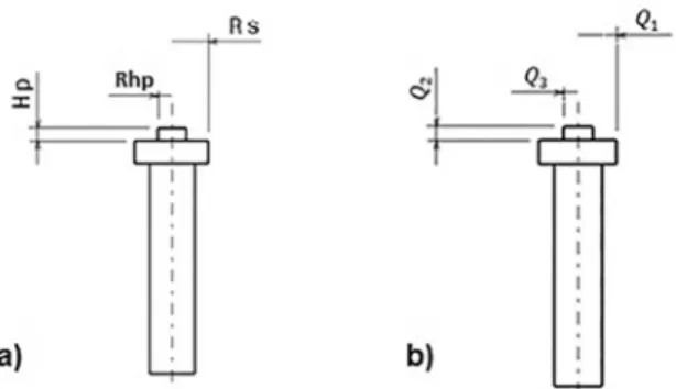
aluminum alloys (e.g. the 2xxx and 7xxx series). After further studies and investigations, the challenge to characterize the principles of FSW and model the evolution of the mechanical and microstructural temperature behavior were developed in large steps by Mishra and Ma3_{. The tool for FSW process} consists of three parts, mounting rod, shoulder and pin, as

shown in Figure 1. Attributed to different functions, the

tool parts do not necessarily need to be machined with the same material. However, if the material is not properly selected, there is high probability of the weld bead not be

efficient and satisfactory visual quality, and tooling wear,

depreciating the tool life4_.

a_{Instituto Tecnológico de Aeronáutica, Praça Marechal Eduardo Gomes, 50, Vila das Acácias,} 12228-900, São José dos Campos, SP, Brasil.

Figure 1. a) Literary dimensions of the cylindrical tool used in the FSW/P. b) Representation of Energies per welding length of each tool interface used in the FSW/P.

Evidence from research around the world, researchers

emphasizes the improvement of benefits when changing the welding process by friction in difficult material to weld and

additive manufacturing5_.

In recent years, numerical models have provided significant

quantitative understanding of the welding processes and welded materials that could not have been possible otherwise. Apart from the calculation of temperature and velocity

fields, these models have been used to calculate various

A Ff v=

Table 1. Chemical composition of alclad 2024-T3 aluminum in (%)7

Si Fe Cu Mn Mg Cr Ni Zn Ti Al

0.5 0.5 3.8-4.9 0.3-0.9 1.2-1.8 0.1 0.5 0.25 0.15 bal

0.17 0.23 4.52 0.59 1.4 0.002 0.0025 0.028 0.013 bal

models have not been widely used, especially in the industry.

An important difficulty is that the model predictions do not

always agree with the experimental results because most phenomenological models lack any built-in component to safeguard the reliability of the model outputs. For example, the computed temperatures do not always agree with the corresponding measured values6_.

In order to study the microstructural changes associated with a FSW aluminum alloy 2024, a model of the material

flow generated during the process has been developed. In this

study, it was considered the forging force along the welding for the energy calculations generated and temperature. By numerically integrating the equations of the model, predictions are obtained for the forces of forgings, welding temperature and energy generated in each step of the process. Knowing

the influence of the energy, force and temperature cycling

behavior of this model is validated in comparison with the experimental procedures.

2. Experimental Procedures

The base material is 1/8 "thickness AA2024-T3 Alclad aluminum alloy with a dimension of 263 x 50 x 3.175 [mm].

The chemical composition of the base material was verified

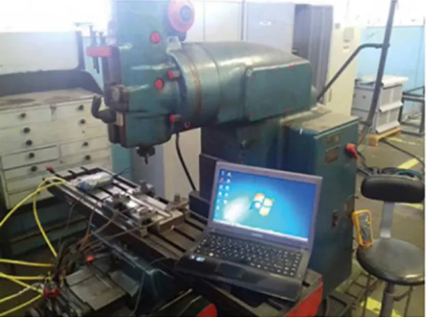
according to Table 1 and compared with the literature7_. The welding tool was manufactured with 15.87 mm of shoulder diameter, 6.4 mm of pin diameter and 2.9 mm of pin height, with cylindrical geometry, exhibited in Figure 1, after machining of the tool it was done thermal treatment in the tool at 1000ºC and quenched in oil, totalizing Hardness from 12 to 55 Rockwell C. The experimental procedure was performed in a vertical milling machine, using the process parameters of 520 rpm of rotation tool speed, 35 mm/min of advance and 2.8 mm of plunging. In order to obtain a good value of parameters, 49 tests were carried out to analyze parameters, K-type thermocouples were used to measure the temperatures in the sample that was welded by the FSW process and electric current in mA of the axial motor that controls the forging force system and were used a multimeter with data acquisition and PC to measure the forging force system, obtained three data by second. Figure 2 shows the temperature data acquisition system and forging force.

2.1 Thermomechanical modeling

To perform the thermomechanical modeling, it was considered Figure 2 for the considerations energy generated in the system, considering a torque dM, angular rotation

ω and transverse velocity of advance ϑ, then results in an

infinitesimal energy generation dQ.

There is also the existence of the nomenclatures according to Table 2, which details all the parameters used for theoretical modeling with their respective unit.

The analytical modeling of heat generation consists of three essential steps in the generation of heat in any tool for

FSW, that are Q1, Q2 and Q3, as shown in Figure 2b. This heat generation is essential for the mechanical properties of friction welding. Some initial considerations are essential for the beginning of modeling:

1. It was considered uniform the contact shear τ_contact; 2. The shear condition will occur at the contact interface 3. Mechanism of heat generation by deformation

was considered

4. Due to friction and shear contact the following cases were considered from the beginning: τ_contact = τ_friction = µp = µσ, being that, ;

5. The forging force was considered from the outset in the initial heat quantities;

6. The area variation between the shoulder and the pin is considered in equations Q₁, Q₂ and Q₃. 7. The physical principle of convection has not been

estimated, but is inherent in the process.

It is considered that the generation of heat generated by a tool of smooth shoulder, cylindrical pin and without radius variation, the quantity of heat generated by a source dQ:

(1)

It is knowns that a segment of area dA is configured by:

(2)

Thus, a constant contact shear segment is obtained. The segment τ_c contributes an infinitesimal force, being:

(3)

And the torque:

(4)

Then, Eq. (5) is written into consideration item IV of the initial considerations:

(5)

Considering the contact of tool surface and workpiece is shown in Figure 2.

*

* *

* *

*

dQ

=

~

dM

=

~

r

dF

f

=

~

r

x

c

dA

*

*

dA

=

r

d

i

dr

*

dF

f

=

x

c

dA

*

dM

=

r

dF

f

* *

*

*

*

*

*

dQ

r

dF

f

r

d

dr

2

~

~

n v

i

Table 2. Contents of the nomenclatures used in thermo mechanical modelling.

Nomenclature Units Description

Q₁ J Heat generation from the shoulder

Q2 J Heat generation from the side probe

Q3 J Heat generation from the surface probe

Q_T J Total heat generation

QE/wl J Energy per unit length of the weld

Q_eff J Effective energy per weld length

τcontact Pa Contact shear stress τfriction Pa Contact friction stress

dQ - Infinitesimal heat generation

dM - Infinitesimal torque

dFf - Infinitesimal forging force dθ - Infinitesimal angular

dA - Infinitesimal area

dr - Infinitesimal radius

σ Pa Contact pressure

F_f kN Forging force

A mm2 _{Tool contact area}

ω rad/s Tool angular rotation speed

R mm Radius

µ - Friction coefficient

Rs mm Tool shoulder radius

R_hp mm Tool probe radius

t mm Thickness workpiece

Hp mm Tool probe height

ϑ m/s Transverse tool speed of ω * r

ρ kg/m3 _density

α W/m*K thermal diffusivity

k W/m*K thermal conductivity

cp J/kg*K specific heat capacity

Figure 2. Data acquisition of FSW process.

2.1.1 Heat generation from the shoulder surface

The heat generation of the shoulder surface starts from the probe surface to shoulder surface, characterized by Q₁.

(6)

(7)

2.1.2 Heat generation of the lateral surface of the cylindrical pin

The lateral heat generation of the pin consists of height l, being H_P, along the radial axis which coincides with the radius of the tool pin R_hp. The heat generation of the pin is obtained by the following equation:

(8)

(9)

(10)

2.1.3 Surface heat generation of the cylindrical pin

Considering a cylindrical pin with constant radius and integrating Eq. (5), thus:

(11)

(12)

Thus, total heat generation constitutes the sum of heat shown in Fig. 2b, coming from Eq. (7), (10) and (12).

(13)

(14)

According to Hamilton et al.8_{, the energy per weld} length is given by the total welding energy, given by Eq. (14), divided by the transverse tool speed. Considering the sliding contact condition observed in item IV in the initial considerations, it is obtained:

(15)

*

*

*

*

*

Q

r

d

dr

Rhp Rs 1 2 0 2

~

n v

i

=

r

#

#

*

*

*

*

Q

R

R

F

R

R

3

2

s hp f s hp 1 2 3 3

~ n

=

-

-Q

V

Q

V

*

*

*

*

*

Q

2

r

2

d

dz

0 1

0 2

~

n v

i

=

r

#

#

*

*

*

*

*

Q

2

H

p

R

₂

hp

2

2

r ~ n v

=

T

Y

*

*

*

Q

2

₂

F

f

H

p

~ n

=

*

*

*

*

*

Q

r

dr

d

R 3 2 0 0 2 hp

~

n v

i

=

r

#

#

*

*

*

*

Q

3

=

₃

2

~ n

F

f

R

hp

Q

T

=

Q

1

+

Q

2

+

Q

3

* * * * Q F R R R R R H 3 2 2 T f s hp s hp hp p 2 3 3 ~ n = -+ +

Q

Q

V

V

#

&

G

J

* * * * Q F R R R R R H 3 2 2 / E wl f s hp s hp hp p 2 3 3 j ~ n = -+ +

Q

Q

V

V

#

&

The effective energy per weld length, according to

Hamilton et al.8_{, is calculated by the ratio of the height of the} pin length H_p and the thickness t of the material multiplied by the energy per weld length.

(16)

For the validation of this model, it was used an empirical equation proposed by Hamilton et al.8_{, that relates the welding}

temperature and the effective energy by the weld length,

which is given by:

(17)

Being α at the diffusivity term,

(18)

2.1.4 Welding surface temperature

In order to ascertain the welding surface temperature during the process, the theoretical method was adopted according to Incropera F. and DeWitt P.9 _{and represented} according to the equations below. The goal of this method is analyze the behavior of the surface temperature of the

process, based on that Δx ≠ Δy and the use of finite difference

equations of the heat equation.

The above representation presents the two-dimensional arrangement, based on the red color are the physical thermocouples and in black the calculated process temperatures.

For the calculation between temperature of the thermocouple T₁ to T₃, there is a heat flow q and a heat flow temperature T_q and based on Figure 3 below which represents the temperatures measured during the welding process, the following correspondents equations.

For the heat flow q1-3:

(19)

For the heat flow temperature T_q1-3:

(20)

Then the process temperature from T₁ to T₃ it is obtained:

(21)

Proceeding for T_q1-2y, there is a variation of displacement between the distances to be measured, therefore, in this

case, ∆x ≠ ∆y.

For the heat flow q1-2y:

(22)

For T_q1-2y, we have:

(23)

Thus, the temperature at the point in question T_1-2y it is obtained:

(24)

The equations for item T_2-3d are thus obtained in an analogous way:

(25)

Then, we have the heat flow temperature equation T_q2-3d:

(26)

Thus, the temperature at the desired point T_2-3d:

(27)

For the point T_2-4, the consideration of ∆y = 0 is used for

the physical effects of the heat flow thermodynamics q2-4.

(28)

For the heat flow temperature of the aforesaid point,

we have: (29)

T

T

y

T

T

T

d

T

T

T

y

T

T

T

d

T

T

T

y

T

1

1 2

2

1 3

2 3

2 4

3

3 4

4

3 5

4 5

4 6

5

5 6

6

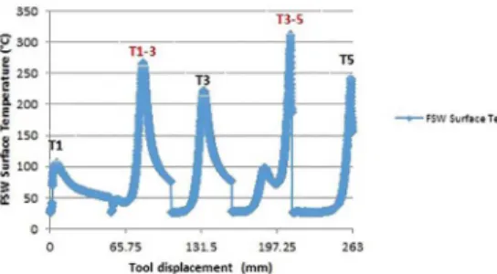
Figure 3. Surface experimental temperatures measured in the welding process FSW.

*

Q

eff

H

_t

Q

/

p

E wl

=

T

Y

*

*

T

T

Q

_R

R

s w eff hp hp

a

n

=

+

*

c

k

p

a

=

_t

q

x

k

T

T

T

2

2

4

1 3 2

_$

1 4 3

D

=

-

-

+

-

Q

V

Q

V

Q

V

T

q1 3

q

₄

_k

x

1 3

_$

D

2

=

-T

1 3

4

T

T

₂

Q

2

T

3 4

=

-

-q

x

k

T

T

T

2

2

4

y

1 2 2

_$

1 3 1 3

D

=

-

-

+

-

Q

V

Q

V

Q

-

V

T

q

k

x

y

q1 2y 1 2y

2

$

D

D

=

-- -

T

R

W

Y

T

y

2

T

T

₂

4

T

q y x

1 2

1 1 2 1 3

=

-

-

+

--

-q

x

k

T

T

T

2

2

4

d y

2 3 2

_$

3 1 1 2

D

=

-

-

+

-

Q

V

Q

V

Q

-

V

T

q

k

x

y

q2 3d 2 3d

2

$

D

D

=

-- -

T

R

W

Y

T

d

2

T

T

₂

4

T

q d

2 3

1 2 3 3

=

-

-

+

-q

x

k

_T

T

T

2

2

4

d

2 4 2

_$

2 4 2 3

D

=

-

-

+

-

Q

V

-T

q2 4

q

₄

_k

x

2 4

_$

D

2

=

-Getting like this:

(30)

Using the same concept of the aforesaid item, the equations for the desired point T_3-5. follow below. For physical effects,

it is considered that ∆y = 0, obtaining a heat flow q3-5:

(31)

And so the temperature of the heat flow T_q3-5:

(32)

And then the point T_3-5:

(33)

Then for the point T_3-4y, it is used the above-mentioned

concept, we have the heat flow q3-4y:

(34)

Obtaining a heat flow temperature:

(35)

Thus:

(36)

Analogously the point T_4-5d with a heat flow q_4-5d:

(37)

Thus the temperature of the heat flow temperature T_q4-5d:

(38)

And then, the desired point T_4-5d:

(39)

For the point T_4-6 it is analogous to the point T_2-4,

considering the same consideration of ∆y = 0 for physical effects of heat flow q4-6.

(40)

And then the heat flow temperature Tq4-6:

(41)

And results in the desired temperature point T_4-6:

(42)

For the last point T_5-6y, the rule that ∆x ≠ ∆y is applied to the physical phenomena already mentioned. For this, the

heat flow equation q_5−6y follows below:

(43)

Thus obtaining a temperature of the heat flow:

(44)

And thus, the last point T_5-6y:

(45)

3. Results and Discussion

3.1 Visual inspection

In order to verify the quality of the welding, the weld

bead was evaluated to ascertain the existence of flashes,

failures due to forging force variation or defects caused by cold weld.

Firstly, a global inspection was performed in the Figure 4,

and micro flashes that made from excess deformed material not retained by the flat surface shoulder, were found due to the hot welding, where the flashes originated, there were

defects caused by the high forging force and variation and a change in the weld bead as explained below.

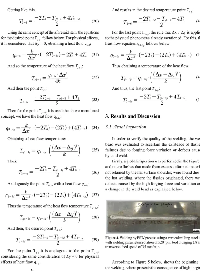
Figure 4. Welding by FSW process using a vertical milling machine with welding parameters rotation of 520 rpm, tool plunging 2.8 and transverse feed speed of 35 mm/min.

According to Figure 5 below, shows the beginning of the welding, where presents the consequence of high forging force, to deform the material and this is evidenced by the presented high visual roughness.

From Figure 6 shows the existence of a linear defect of 28.4 mm in extension, originated by the high forging force

variation in the geometry of the flat bottom shoulder tool,

as consequence a strain variation, causing the linear defect.

T

2 4

2

T

T

q

₂

4

T

d

4 2 4 2 3

=

-

-

+

--

-q

x

k

_T

T

T

2

x

2

4

3 5 2

_$

2 4 5 3

D

=

-

-

+

-

Q

-

V

T

q3 5

q

₄

_k

x

3 5

_$

D

2

=

-T

3 5

2

T

₂

T

q

4

T

2 4 3 5 3

=

-

-

+

--

-q

x

k

T

T

T

2

2

4

y

3 4 2

_$

3 4 3 5

D

=

-

-

+

-

Q

V

Q

V

Q

-

V

T

q

k

x

y

q3 4y 3 4y

2

$

D

D

=

-- -

T

R

W

Y

T

y

2

T

T

₂

4

T

q y

3 4

3 3 4 3 5

=

-

-

+

--

-q

x

k

T

T

T

2

2

4

d y

4 5 2

_$

3 5 3 4

D

=

-

-

+

-

Q

V

Q

V

Q

-

V

T

q

k

x

y

q4 5d 4 5d

2

$

D

D

=

-- -

T

R

W

Y

T

d

2

T

T

₂

4

T

q d y

4 5

3 5 4 5 3 4

=

-

-

+

-- -

-q

x

k

T

T

T

2

2

d

4

4 6 2

_$

4 4 5 6

D

=

-

-

+

-

Q

V

-T

k

q

x

4

q4 6

4 6

_$

D

2

=

-T

4 6

2

T

d

₂

T

q

4

T

4 5 4 6 6

=

-

-

+

--

-q

x

k

T

T

T

2

2

4

y

5 6 2

_$

3 5 3 5

D

=

-

-

+

-

Q

V

Q

V

Q

-

V

T

q

k

x

y

q5 6y 5 6y

2

$

D

D

=

-- -

T

R

W

Y

T

y

2

T

T

₂

4

T

q y

5 6

5 5 6 3 5

=

-

-

+

-Figure 5. FSW welding start, high forging force and roughness.

Figure 6. Linear defect with 28.4 mm extension, from cold welding, due to high variation in forging force.

According to Figure 7, at the end of the welding, there was a variation of 18.37% in the diameter of the weld bead,

this variation was originated by low stiffness and clearance

that the vertical milling machine additionally provided a variation in the forging force causing a roughness change at the end of the welding process.

Figure 7. Variation in the final diameter of the weld bead of 18.37%,

originated by the lack of rigidity of the vertical milling machine and high forging force variation at the end of the process.

3.2 Forging force analysis

The graph in the Figure 8 shows the forging force during the FSW process, obtaining an average forging force of 0.774 kN.

The high forging force presented in the first sector of

the graph is characterized by the low thermal input at the

Figure 8. Forging force in the FSW process with a mean of 0.774 kN.

beginning of the process, consequently the high forging force, reaching 0.883 kN. The high particle size is also presented at the beginning of the welding, according to Figure 5.

The correlation between Figure 6 shows linear defects from the hot weld by high irregular deformation in the material and the second stage of the graph presented is the high variation of this forging force together with the low rigidity of the vertical milling machine.

The low stiffness of the vertical milling machine is also

evident in Figure 8 by the high variation in forging force at the end of the FSW process, characterized by visual inspection in Figure 7.

3.3 Theoretical energy analysis and surface

welding temperature

As show in Figure 3, the same corresponds to the temperatures measured in the FSW process execution. Initiating the process without the use of dwell time, the low

thermal input in the first two channels (CH1 and CH2) it's evident. However, the rate of heat flow tends to increase

with the higher generation of friction and deformation, consequently, the temperature of the CH2, increases when the tool passes through the half of the process, distance of approximately 131.5 mm and with the physical phenomena of thermodynamics gets the absence of heat until stabilization at the end of the process.

At the temperature of CH3 there is an onset of temperature increase when the tool passes in the 102.5 mm and persists up to the maximum of 185.5 mm, in this channel the phenomenon of heat convection is present after the maximum temperature of the point. The temperature of the CH4 accompanying the temperature of the CH3 as well as the conduction of heat of the CH2, it is realized that when the temperature of the CH2 increases, the temperature of the CH4 also increases by conduction of heat, the three channels being CH2, CH3 and CH4 are stimulated by conduction and convection at almost the same point.

and greater thermal input present at the end of the process. However, the CH6 temperature value is present from a lower temperature peak among all measured temperature peaks, whereby the high convection of the aluminum in the FSW process it is evident.

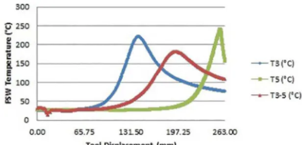
The analytical temperature T_1-3 was calculated according to equations 19, 20 and 21. The comparison between temperature gradient T₁ and T₃ in the Figure 9, it is carried out, they are coherent with the dimensional state between the two temperatures. Physically, there is a state of temperature higher than the temperature T₁ and T₃ and it explains the conduction phenomenon and the high level of

energy generated to effect the welding process by FSW the

analytical value of T_1-3.

position where it is positioned. At this point the physical principles of thermodynamics add to a curve disposition between logically measured values when the tool passes through the point, the conduction of heat is evidenced due to the points are equidistant and due to a special attention at the intersections of lines between the temperatures T₁; T_2-3d

and T_2-3d; T₃, all of them show a rise at their intersections, which represents the positive interaction of the analytical model in respect to the temperature measured T₁ and T₃.

Figure 9. Welding analytical surface temperature T1-3

From Figure 10 it is represented by the analytical calculation of temperature T_1-2y under Equations 22, 23 and 24. In comparison with the distance between the temperatures

T₁ and T_1-3, they are in logical dimensional state with the arrangement of the calculation and the adjacent temperatures. The constants resulting from this analytical mode are present by the steps shown in the temperature curve T_1-2y, these constants are inherent to the process, exhibit acute temperature shifts and a high heat dissipation it is evidenced by the constant k of the material.

Figure 10. Welding analytical surface temperature T1-2y.

From Figure 11 this analytical representation with respect to the temperature T_2-3d and Equations 25, 26 and 27, the distance between the temperatures T₁ and T₃ deals in a coherent way in respect to the value in relation to the

Figure 11. Welding analytical surface temperature T2-3d.

From Figure 12 shows the analytical temperature curve

T_2-4 together with the experimental temperature curves T₂

and T₄, the analytical temperature related to the experimental temperatures are in dimensional coherence. The heat transfer attributed at this analytical temperature is related to the conduction of heat that the material provides in relation to the heat that the tool provides by the deformation and the generated friction.

Figure 12. Welding analytical surface temperature T2-4.

Figure 13 shows the relationship in between the analytical temperature T_3-5 and the experimental temperatures T₂ and

T₄ is in dimensional coherence. The physical reasons for heat transfers take special note in this case between the intersections of lines between the experimental curves and the analytical curve that the physical principle of conduction shows a rise at their intersections which represents the positive interaction of analytical modeling with respect the temperature measured T₂ and T₄.

The dimensional interaction between the analytical temperature T_3-4y and the experimental temperatures T₃ and

Figure 13. Welding analytical surface temperature T3-5.

Figure 14. Welding analytical surface temperature T3-4y.

Figure 15. Welding analytical surface temperature T4-5d.

Figure 16. Welding analytical surface temperature T4-6.

the point in question. Physically in the Figure 14 has a heat dissipation by the k factor of the material when it is in a state of high thermal input causes the temperature at this point to be greater than the temperature T₄ and less than T₃.

From Figure 15 the interaction of heat transfer factors between the analytical temperature T_4-5d it is seen as a sum

of dependencies of heat flow generated by the experimental

temperatures T₃ and T₅ with the analytical temperature T_4−5d. In the dimensional point of view, the curve is consistent with the analytical dimension. Physically, the amount of heat

flow from the adjacent temperatures that is needed to do the

analytical modeling becomes evident, the temperature rise

by approximately 150 mm is dependent on the heat flow of

the analytical temperature T_3-4y and the analytical temperature

T₃, After the loss of heat flow through conduction, between

180 mm and 235 mm, the heat flow returns to positive result

due to the high experimental temperature T₅.

Figure 16 presents again a typical case in which the heat transfer parameters are constants that are analytically inherent to the process, shows temperature shift at the end of the process and high heat dissipation is evidenced by the constant k of the material. Dimensionally, the analytical curve presents in coherence with the displacement of the tool in relation to the measured analytical point.

Figure 17. Welding analytical surface temperature T5-6y.

According to Figure 17, the analytical temperature T_5-6y

is in dimensional agreement with the temperature T₅ and T

5-6y. The heat conduction generated by the temperature flow T_3-5 provided the first temperature accumulation step and its

stabilization until the beginning of the heat conduction of the temperature T₅, with this there was a vast gain of heat

flow, directed at the way the temperature T_5-6y had the same behavior as T₅.

For a better understanding of what happens when the tool moves in the forward direction, the graphs exhibited in Figure 18 and 19 are considered. The amount of energy used for welding in relation to the temperature at the beginning of the process is evidenced as inversely proportional, this reason is explained by the low thermal input that is generated at the beginning of the process, causing a greater forging force and

greater effective energy per weld length to start the process,

Figure 18. Analytical and experimental surface welding temperature in FSW process.

Figure 19. Theorical and Experimental Qeff

Figure 19 due to the excellent thermal conductivity of the material and the thermal input generated during the process even with temperature oscillations, As shown in Figure 18, during the analytical temperatures T_1-3 and T_3-5 with the measured temperatures T₁, T₃ and T₅.

4. Conclusions

In this work, a theoretical model was developed with the objective of measuring the energy per unit length of the welding process (Friction Stir Welding) that uses the forging force from the shoulder of the welding tool as a main parameter for this analysis. Additionally a cylinder pin geometry tool was assigned for the calculations presented. In addition, a two-dimensional model of temperature modeling

was presented, given Δx and Δy and six temperature points

measured.

The equations developed for the surface welding temperatures presented coherent when compared with the values measured by the thermocouples that were placed along the weld bead. This was observed both in the dimensional analysis of tool displacement and in the results of the intensity of these analytical temperatures and can be used for any temperature measurement points.

In the development of the equations for energy by welding length, new parameters functions were attributed that serve as the basis for this modeling, and a predominant factor of the process was the inclusion in theoretical modeling of the forging force generated by the tool shoulder. In the

development of the equations for energy by welding length, new parameters functions were attributed that serve as the basis for this modeling, and a predominant factor of the process was the inclusion in theoretical modeling of the forging force generated by the tool shoulder. In this way, the energy values obtained from the theoretical modeling can be compared with the forging forces applied by the

shoulder of the tool reflecting in the FSW welding process.

It is can be seen from the visual inspection that the variation of forging force is a predominant factor in the manifestation of the linear defects and high roughness of the weld bead.

In this context, the proposed theoretical energy model presented in this paper consists of an auxiliary tool of the welding process using the FSW, leaving it more reliable. With industrial competitiveness the process energy modeling it is fundamental to analyze news parameters variations, rotation, plunge and transverse tool speed, making the process more reliable, minimizing the possible defects that can arise.

5. Acknowledgement

Our sincere acknowledgements to the Technological Institute of Aeronautics for teaching support and Embraer for the donation of alclad aluminum alloy AA2024-T3.

6. References

1. M.W. Mahoney, Science Friction, Weld. Join., Jan/Feb 1997, p 18-20.

2. Thomas WM, Nicholas ED, Needham JC, Murch MG, Temple-Smith P, Dawes CJ, inventors. Friction Stir Butt Welding. International Patent Application PCT/GB92/02203. GB Patent Application 9125978.8.1991 Dec.

3. Mishra RS, Ma ZY. Friction stir welding and processing. Material

Science and Engineering: R: Reports. 2005;50(1-2):1-78.

4. Threadgill PL. A review of Friction Stir Welding: Part 2, selection of materials toll. Cambridge: The Welding Institute; 2003.

5. Rao KP. Friction surfacing - a versatile technique. Prof. Dr. DRG Achar, memorial award for distinguished academician

lecture. Tiruchirappalli: Indian Welding Society; 2011. 12 p.

6. Mishra S, DebRoy T. A heat-transfer and fluid-flow-based model to obtain a specific weld geometry using various

combinations of welding variables. Journal of Applied Physics. 2005;98(4):044902.

7. Davis JF; ASM International Handbook Committee. ASM Handbook Volume 2: Properties and Selection - Nonferrous

alloys and Special-Purpose materials. 10th _{ed. Metals Park:}

ASM International; 1990.

8. Hamilton C, Dymek S, Sommers A. A thermal model of friction stir welding in aluminum alloys. International Journal of

Machine Tools and Manufacture. 2008;48(10):1120-1130.

9. Incropera FP, DeWitt DP. Fundamentals of Heat and Mass