João Luiz F. Azevedo* Institute of Aeronautics and Space São José dos Campos – Brazil
Heidi Korzenowski VSE- Vale Solutions in Energy São José dos Campos – Brazil [email protected]
*author for correpondence
An assessment of unstructured
grid inite volume schemes
for cold gas hypersonic low
calculations
Abstract: A comparison of ive different spatial discretization schemes is
performed considering a typical high speed low application. Flowields are simulated using the 2-D Euler equations, discretized in a cell-centered inite volume procedure on unstructured triangular meshes. The algorithms studied include a central difference-type scheme, and 1st- and 2nd-order van Leer and Liou lux-vector splitting schemes. These methods are implemented in an eficient, edge-based, unstructured grid procedure which allows for adaptive mesh reinement based on low property gradients. Details of the unstructured grid implementation of the methods are presented together with a discussion of the data structure and of the adaptive reinement strategy. The application of interest is the cold gas low through a typical hypersonic inlet. Results for different entrance Mach numbers and mesh topologies are discussed in order to assess the comparative performance of the various spatial discretization schemes.
Keywords: Hypersonic low, Cold gas low, Finite volume method, Unstructured
grids, Spatial discretization schemes.
INTRODUCTION
The present work considers that the lowields of
interest are simulated using the 2-D Euler equations. For such hyperbolic equations, the physical propagation of perturbations occurs along characteristic lines. The schemes based on central spatial discretizations possess symmetry with respect to a change in sign of the Jacobian matrix eigenvalues which does not distinguish upstream
from downstream inluences. In such case, these schemes do not consider physical properties of the low equations
into the discretized formulation and this generates oscillations in the vicinity of discontinuities which have to
be damped by the addition of artiicial dissipation terms.
The problem is, therefore, to determine the adequate
amount of artiicial dissipation which should be large
enough to damp instabilities and, at the same time, small
enough to avoid the destruction of low features.
Upwind schemes take into account physical properties in the discretization process and they have the advantage of being naturally dissipative. Flux vector splitting methods introduce the information of the sign of the eigenvalues
in the discretization process, and the lux terms are split
and discretized according to the sign of the associated propagation speeds. Steger and Warming (see, for instance, Steger and Warming, 1981, and Hirsch, 1990) make use
of the homogeneous property of the Euler equations
and split the lux vectors into forward and backward
contributions by splitting the eigenvalues of the Jacobian matrix into non-negative and non-positive groups. The
split lux contributions are, then, spatially differentiated
according to one-sided upwind discretizations. However,
these forward and backward luxes are not differentiable
when an eigenvalue changes sign, and this can produce
oscillations at sonic points. In order to avoid these
oscillations, van Leer (1982) determines a continuously
spatially differenced lux vector splitting that leads to
smoother solutions at sonic points.
In the present work, the interface luxes are calculated using ive different algorithms, including a central difference-type scheme, and van Leer (1982) and Liou (1996) lux vector splitting schemes. In the central difference case, the interface luxes are obtained from an average vector
of conserved variables at the interface, which is calculated by straightforward arithmetic averages of the vector of conserved variables on both sides of the interface. Since this approach provides no numerical dissipation terms to control nonlinear instabilities, an appropriate blend of undivided Laplacian and biharmonic operators is explicitly
added as the necessary artiicial dissipation terms. For the irst-order van Leer scheme, the interface luxes are
obtained by van Leer’s formulas (van Leer, 1982) and they are constructed using the conserved properties for the i-th control volume and its neighbor across the given
interface. The second order scheme considers a MUSCL approach (Anderson, Thomas and van Leer, 1986), that is,
the interface luxes are formed using left and right states at
the interface, which are linearly reconstructed by primitive variable extrapolation on each side of the interface. The extrapolation process is effected by a limiter in order to
avoid the creation of new local extrema. The irst- and
second-order Liou schemes consider that the convective operator can be written as a sum of the convective and pressure terms (Liou, 1996). The second-order scheme also considers a MUSCL approach.
The Euler equations are discretized in a cell-centered
inite-volume-based procedure on unstructured triangular meshes.
Time march uses a fully explicit, 2nd-order accurate,
ive-stage Runge-Kutta time stepping scheme. Only steady-state calculations have been considered in the present context, and variable time stepping and implicit residual smoothing procedures have been employed to accelerate
convergence to steady-state. Computations using a ine, ixed, unstructured mesh are compared to those obtained
with an adaptive mesh procedure in order to assess the quality of the solutions calculated by the different schemes
implemented and in order to analyze the mesh inluence in the capture of the low features of interest.
The schemes discussed here are applied to the solution of
supersonic/hypersonic inlet lows. A 2-D inlet conigu-
ration which is representative of some proposed inlet geometries for a typical transatmospheric vehicle is considered. The inlet entrance conditions were varied
from a freestream Mach number M∞ = 4 up to M∞ = 16
in order to test the schemes implemented for a wide
range of possible inlet operating conditions. The luid
was treated as a perfect gas and, hence, no chemistry was taken into account. From a physical standpoint, the
present simulations are typical of cold gas lows which
are usually achieved in experimental facilities such as gun tunnels. This is certainly not representative of actual
light conditions in which dissociation and vibrational
relaxation are important phenomena, especially for the higher Mach number cases. However, it is a necessary step in order to construct a robust code to deal with the
complete environment encountered in actual light.
THEORETICAL FORMULATION
The 2-D time dependent Euler equations can be written in integral form as
, (1)
where P→= Eî + Fĵ. The application of the divergence
theorem to Eq. (1) will yield
, (2)
where V represents the area of the control volume, S is its
boundary and n→ is the outward normal to the S boundary.
The vector of conserved quantities, Q, and the convective
lux vectors, E and F , are given by
, (3)
. (4)
Here, ρ denotes the density, p is the pressure, u and v
represent the Cartesian velocity components, and e is the total energy per unit of volume.
If the equations are discretized using a cell-centered
inite-volume-based procedure, the discrete vector of conserved
variables, Qi , is deined as an average over the i-th control
volume as
. (5)
In this context, the discrete low variables can be assumed
as attributed to the centroid of each cell if necessary. With
the previous deinition of Qi , Eq. (2) can be rewritten for the i-th volume as
. (6)
SPATIAL DISCRETIZATION ALGORITHMS
Spatial discretization is essentially concerned with
inding a discrete approximation to the surface integral in Eq. (6). This approximation is the so-called convective operator, C (Qi), i.e.,
. (7)
Centered Scheme
In the centered scheme case, the convective operator is
deined as
. (8)
interface, where i is the i-th control volume and k is its
neighbor. The terms ∆xik and ∆yik are calculated as
, (9)
where the points (xk1 , yk1) and (xk2 , yk2) are the vertices
which deine the interface between cells i and k (Azevedo,
1992).
The spatial discretization procedure presented in Eq. (8) is equivalent to a central difference scheme. Therefore,
artiicial dissipation terms must be added in order to control
nonlinear instabilities (Jameson and Mavriplis, 1986).
In the present case, the artiicial dissipation operator, D(Qi), is formed as a blend of undivided Laplacian and biharmonic operators (Mavriplis, 1988, and Mavriplis, 1990). These mimic, in an unstructured mesh context, the concept of using second and fourth difference terms (Jameson, Schmidt and Turkel, 1981, and Pulliam, 1986).
Therefore, the artiicial dissipation operator is given by
, (10)
where d(2)(Qi ) represents the contribution of the
Laplacian operator and d(4) (Q
i ) represents the
contribution of biharmonic operator.
In order to form the biharmonic operator, it is necessary to irst deine the undivided Laplacian operator for the i-th control volume as
, (11)
where the summation in k is taken over all control volumes
which have a common interface with the i-th cell. The
biharmonic operator is, then, deined as (Azevedo, 1992,
and Azevedo and Oliveira, 1994)
(12)
The Laplacian operator is responsible for avoiding oscillations near discontinuities and it is constructed as
. (13)
Here, the coeficient єik
(2) is given by
, (14)
where the switching function νi is deined in terms of the
local pressure gradient as
. (15)
Close to discontinuities, the biharmonic operator produces
oscillations. Therefore, the coeficient єik(4) is deined
such that it is switched off when the second difference
coeficient, єik(2) , becomes large. This typically occurs
near shocks or other discontinuities. The єik(4) coeficient is deined as
. (16)
Typical values for the constants (Mavriplis, 1988) are K(2)
= 1/4 and K(4) = 3/256.
First-Order Van Leer Scheme
The convective operator, C (Qi ), is deined for the van
Leer lux vector splitting scheme (van Leer, 1982, and Anderson, Thomas and van Leer, 1986) by the expression
, (17)
where ∆xik and ∆yikare given by Eq. (9). In the present
case, the interface luxes, Eik and Fik, are deined as
(Azevedo and Figueira da Silva, 1997)
,
(18) .
Here, Ei± and F i
± are the split luxes calculated using van
Leer’s formulas (van Leer, 1982, and Anderson, Thomas and van Leer, 1986) and the conserved properties of the i-th control volume. The evaluation of the split luxes in the van Leer context can be summarized as follows:
.
(19)
In the previous equations, the Mach number in the x-direction is deined as Mx = u/a and the split mass
luxes are f± = ±ρa [(M
x± 1) /2]2 . Similar expressions
are obtained for F± using M
y = v/a. With this lux vector deinition, the splitting is continuously differentiable at
Second-Order Van Leer Scheme
In the present work, the implementation of the 2nd-order
van Leer scheme is based on an extension of the Godunov approach. The projection stage of the Godunov scheme, in which the solution is projected in each cell on piecewise
constant states, is modiied. This constitutes the so-called
MUSCL (Monotone Upstream-Centered Scheme for Conservation Laws) approach (van Leer, 1979) for the extrapolation of primitive variables. By this approach, left and right states at a given interface are linearly reconstructed by primitive variable extrapolation on each side of the interface, together with some appropriate limiting process (Hirsch, 1990) in order to avoid the generation of new extrema. The vector of primitive variables is taken as W = [p, u, v, T ]T , in the present
case. The convective operator, C (Qi ), can be deined as
indicated in Eq. (17). The interface luxes, Eik and Fik , are deined as
, ,
(20)
where QL = Q(WL ) and QR = Q(WR ) are the left and right
states at the ik interface obtained by the linear extrapolation process previously discussed.
There are two aspects of the unstructured grid implementation of such a scheme which deserve further
consideration. The irst aspect concerns the deinition of
“left” and “right” states at a given cell interface. Since there is no concept similar to curvilinear coordinates in this case, the cell interfaces can have virtually any orientation and one must decide which way to “look” in order to construct left and right states. This is done in the present case based on the components of the vector normal to the edge, as already indicated in Eq. (18) for the 1st-order van Leer scheme. The other aspect is associated with deciding which second control volume will be used for the reconstruction process in addition to the volume immediately adjacent to the interface considered. The authors emphasize that an edge-based data structure (Mavriplis, 1988) is being used in this development and further discussion of the data structure used will be presented later in the paper.
The procedure adopted in the present case to handle the second aspect is inspired by the work of Lyra (1994). The major difference between the present implementation and the cited reference lies in the direction in which the
one-dimensional stencil is constructed. In Lyra (1994), the
stencil for extrapolation is constructed along the direction
of the edge. It must be emphasized that Lyra (1994) is working with a inite element approach. Here, since a cell-centered inite volume method is of interest, the
extrapolation stencil is constructed in a direction normal
to the edge. In an attempt to reinterpret the 1-D ideas
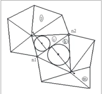
in the present unstructured grid context, a line is drawn normal to the edge and passing through the center of the inscribed circle. A third point is located over this line at a distance from the center of the inscribed circle equal
to the diameter of the circle. The code, then, identiies in
which control volume this 3rd point lies, and it uses the properties of this triangle in the linear reconstruction of the primitive variables.
In order to make the nomenclature clear, the two triangles
which are adjacent to the edge under consideration are
denoted i and k. The second triangle identiied by the
previously described process and associated with triangle i is denoted l. The corresponding one associated with k is denoted triangle m. This is illustrated in Fig. 1. Therefore,
in the calculation of the E± luxes, the left state, Q
L , is deined using the properties of the i and l triangles and the right state, QR , is deined using those of the k and m triangles, if ∆yik ≥ 0. The reverse is true if ∆yik < 0.
Similarly, the deinition of the F± luxes uses data at the i
and l triangles to deine the left state and data at the k and m triangles to deine the right state if ∆xik≤ 0, and vice-versa if ∆xik > 0.
Figure 1: Sketch of the extrapolation stencil used for primi-tive variable linear reconstruction in the 2nd-order upwind schemes.
With the procedure just described, the state variables are represented as piecewise linear within each cell, instead of piecewise constant. But even considering a 2nd-order
lux vector splitting scheme with a MUSCL approach, it is
possible to obtain oscillations in the solution. Therefore one must use nonlinear corrections, namely limiters, to avoid
limiter (Hirsch, 1990) is adopted. Previous experience (Azevedo and Figueira da Silva, 1997) with other limiters, such as the van Leer, van Albada and superbee limiters have indicated that these may not reach machine zero convergence in some cases. On the other hand, the minmod limiter was always able to drive convergence to machine zero in the cases tested in Azevedo and Figueira da Silva (1997) and it was, therefore, the limiter chosen
for the present study. In order to obtain the expression for
the limiter, one has to compute the ratios of consecutive
variations. The limiter will be deined as a function of these ratios. Hence, if one deines
,
(21) ,
the limiters, which will be denoted by φ− and φ+ , can be
written in the minmod case as
(22)
With the previous deinitions, the left and right states at
the interface can be written as:
(23)
The functions F− and F+ reconstruct, respectively, the WL
and WR states, and they are given by
,
(24)
,
where φ− and φ+ are the limiters previously deined.
First-and Second-Order Liou Schemes
The Liou schemes implemented in this work consider that the convective operator can be expressed as a sum of
the convective and pressure terms (Liou, 1994, and Liou,
1996). The inviscid lux vectors can be written as
,
,
(25)
where the Φ, Px and Py vectors are deined as
. (26)
In the previous expressions, p is the pressure, H is the total
speciic enthalpy, Mx = u/a, and My = v/a.
The approach followed in the present work in order to extend Liou’s ideas (Liou, 1994) to the unstructured grid case
consists of deining a local one-dimensional stencil normal
to the edge considered. The reason for this can be perceived if one observes, based on Eq. (17), that the contribution of the ik edge to the convective operator can be written as
. (27)
where the normal n→ik to the ik edge, positive outwards with
respect to the i-th triangle, is deined as
. (28)
Here, ℓik is the length of the ik edge. Hence, one can write
. (29)
where, for now, it is suficient to write Fik (c) and P
ik as
. (30)
For the construction of the irst-order scheme, one must
identify the “left” (or L) state, as deined in Liou (1994,
1996), as the properties of the i-th triangle and the
“right” (or R) state as those of the k-th triangle (see
Fig. 1 for the geometry deinition). Hence, the interface
Mach number, Mik , also according to the deinition in
Liou (1994, 1996), can be written as
, (31)
where ML+ = M+ (ML ) and MR− = M−(MR ). The split Mach
, (32)
and, similarly,
, (33)
The Mβ± terms can be written as
. (34)
The present work used β = 1/8, as suggested in Liou (1994).
Moreover, in order to achieve a unique splitting in Liou’s
sense, the left and right Mach numbers are deined as
, (35)
where
, .
(36)
The corresponding speed of sound, aik, at the interface is
given by
, (37)
where
,
(38)
and a similar deinition for ãR. The pressure, pik, at the ik interface is given by
. (39)
The split pressures, still following the expressions in Liou (1994, 1996), can be written as
, (40)
and, similarly,
, (41)
The pα± terms can be written as
. (42)
This work used α = 3/16, as suggested in Liou (1994).
The convective operator, as deined in Eq. (17), can be
inally written as
, (43)
where
(44)
and Pik has already been deined in Eq. (30). The second order scheme follows exactly the same formulation, except that the left and right states are obtained by a MUSCL extrapolation of primitive variables as described
in the previous section. Therefore, the left state is deined
by a limited extrapolation of the properties in the i-th and
l-th triangles, and the right state is deined by a limited
extrapolation of the properties in the k-th and m-th
triangles. The minmod limiter was again used in this case.
TIME DISCRETIZATION
The Euler equations, fully discretized in space and assuming a stationary mesh, can be written as
, (45)
where the D(Qi ) operator is identically zero if an upwind
spatial discretization is used. The present work uses a fully explicit, 2nd-order accurate, 5-stage Runge-Kutta time-stepping scheme (Mavriplis, 1988) to advance the solution of the governing equations in time. The time integration scheme can, therefore, be written as
,
,
,
(46)
where the superscripts n and n + 1 indicate that these are
property values at the beginning and at the end of the n-th
time step. The values used for the α coeficients were
. (47)
It should be observed that the convective operator, C (Q), is evaluated at every stage of the integration process, but
in order to accelerate convergence. The details of the implementation of the variable time step option can be found in Azevedo and Figueira da Silva (1997).
DATA STRUCTURES
In a cell-centered inite volume context, the standard procedure for lux calculation consists of a loop over
the control volumes which adds up the contribution
of each edge, or side, to form the lux balance for that
particular volume. This is usually called a volume-based data structure, which is the equivalent in the present case
of an element-based data structure for the inite element
community. Although “natural” and straightforward
to implement, this procedure is not the most eficient because luxes end up being computed twice for each
edge of the control volume. For an explicit scheme, this means that the code could theoretically run twice as fast simply by implementing some procedure that would avoid
recomputing the luxes for the same edge.
One of the possibilities for solving this problem is to implement a so-called edge-based (or side-based) data
structure (Mavriplis, 1988). In this case, the idea is to
index the code computations based on the control volume edges. The discussion presented here considers a triangular unstructured grid. However, a similar procedure could be implemented regardless of the type of control volume used. The connectivity information for a cell-centered
inite volume algorithm on a volume-based data structure consists of two major “tables.” The irst one indicates,
for each triangle, the nodes of the mesh which form the triangle. The other table points to the three triangles which are neighbors of the particular triangle considered. For an edge-based data structure, the connectivity information is centered on the edges and, for each edge, enough information should be stored to allow the necessary computations over the complete grid.
In the present work, since a cell-centered scheme is being
used, the following procedure is adopted:
For each edges store: (n1, n2, i, k) . (48)
Here, n1 and n2are the two nodes which deine the edge, i
is the triangle to the left of the n1n2 segment, and k is the
triangle to the right of it (see Fig. 1 for details). Moreover,
the n1n2 segment is assumed to be oriented from n1 to n2 .
This notion of orientation of a segment is fundamental to the algorithm because, with the present implementation,
the nodes n1 and n2 are arranged in a counterclockwise
fashion for the i-th control volume and in a clockwise
fashion for the k-th control volume. Therefore, the lux
computed for this particular edge is added to the lux
balance equation of the i-th control volume and subtracted
from that of the k-th control volume. Hence, for an edge-based data structure, the main loop runs over edges, or sides, and the contribution of the side to the neighboring control volumes is computed and added (or subtracted) to
(from) that volume’s lux balance equation.
The previous information would be enough for the
centered scheme and for the irst-order upwind schemes
implemented here. However, as already discussed, further information is necessary in order to implement the order versions of the upwind schemes. For the second-order upwind schemes, the edge-based information stored must be augmented in order to also include the
identiication of the two additional triangles which are
used for the linear reconstruction process. Hence, using
the nomenclature previously deined, one should:
For each edges store: (n1, n2, i, k, l, m) . (49)
The procedure used to deine triangles l and m has already been previously described in the paper. The search operations necessary to identify these triangles are performed at a pre-processing stage, such that the computational cost associated with this search is negligible
in the overall solution cost. It should be emphasized
that this identiication must also be performed after
each adaptive reinement pass, since the complete
connectivity information is updated in the reinement
process.
ADAPTIVE GRID REFINEMENT
The concept behind using an adaptive mesh strategy is
to reine regions where large gradients occur. For many problems, the regions that need to be reined are small
compared with the size of the complete computational domain. Therefore, one can reduce storage and CPU
requirements by the use of adaptive reinement, when compared with a ixed ine mesh which would yield the same resolution of the relevant low features. In order to identify the regions that require grid reinement, a sensor must be deined. The sensor used in this work is based on gradients of low properties. Its general deinition could
be expressed as
, (50)
and φnmax and φnmin are the maximum and the minimum
values of the φn property in the lowield. Despite this
general deinition, and despite having implemented the
equation, all results presented in this work have used a
sensor based on density gradients, i.e., φn = ρ.
The irst step of the adaptive procedure is to compute the low on an existing coarse mesh. With this preliminary
solution, one can calculate the sensor as previously described. The code marks all triangles in which the
sensor exceeds some speciied threshold value (the threshold value will be denoted Γ in the present paper), and the marked triangles are reined. A new iner mesh is
then constructed by enrichment of the original coarse grid.
The mesh enrichment procedure consists of introducing an additional node for each side of a triangle marked
for reinement. For interior sides, this additional node is
placed at the mid-point of the side whereas, for boundary
sides, it is necessary to refer to the boundary deinition to
ensure that the new node is placed on the true boundary. After this initial pass, the code has to search all triangles to identify cells that have two or three divided sides. Each of these cells is subdivided into four new triangles. This subdivision may eventually mark new faces. Therefore, this process has to be performed until there are no triangles
with more than one marked face. In order to avoid hanging
nodes, the triangles that have one marked face should be divided by halving. Figure 2 illustrates the three possible ways of triangle subdivision.
The second part of the reinement process consists of identifying all triangles which were reined by halving. This information is stored for the next reinement step
because, if there is again an attempt to subdivide these triangles by halving, this is not allowed. Experience has shown that repeated triangle division by halving has a strong detrimental effect in mesh quality. Therefore, if the
next reinement step tries to divide by halving a triangle
which was obtained by halving from a previous division, the logic in the code forces the original triangle to be
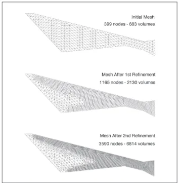
Figure 3: Initial and intermediate grids in the adaptive reine
-ment procedure. Figure 2: Schematic representation of the three possible
trian-gle subdivision processes.
divided into four new triangles before the reinement
procedure is allowed to continue. When the mesh enrichment procedure has been completed, the new control volumes receive the property values of their
“father” triangle and the low solver is re-started.
RESULTS AND DISCUSSION
A 2-D inlet coniguration which is representative of some
proposed inlet geometries for a typical transatmospheric vehicle was used as a test in the present work. To analyze the different schemes, an adaptive mesh and both a coarse
and a ine ixed unstructured meshes were used. In the
present work, the expression “ixed” mesh will denote a
grid which was generated as close as possible to an equally spaced mesh in the unstructured context. Therefore, the
expression “ixed grid” is being used here in opposition to the expression “adaptively reined” grid. The adaptive mesh was obtained with 3 passes of reinement using the 1st-order Liou scheme as the low solver. The adaptive reinement
process described in the previous section was used and the sensor was based on density gradients. The initial mesh had
399 nodes and 683 triangles. The successive reinement passes used threshold values Γ =(0.005, 0.005, 0.005). This
mesh ended up with 11152 nodes and 21692 volumes. The initial mesh and the two intermediate meshes in this process
are shown in Fig. 3. In the present case, 500 iterations were performed before the irst reinement pass, 800 iterations between the irst and the second ones, and 1200 iterations between the second and the third reinement passes. This
in the sense that the optimal number of iterations between
successive reinement passes increases as the grid is reined. The inal mesh is shown as the bottom plot in Fig. 4. This is the adaptively reined grid which was used for comparison
of the various schemes in the paper.
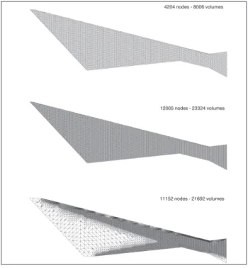
The coarse ixed grid had 4204 nodes and 8006 volumes.
Results for coarser grids were also obtained, but these results were deemed either excessively poor for the purpose of the present comparisons or of comparable resolution with the ones obtained with the above referred
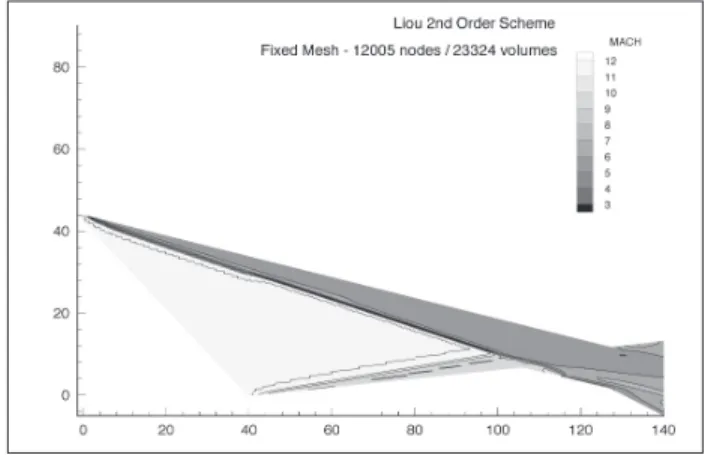
grid. A ine ixed mesh was also generated and this grid had
12005 nodes and 23324 triangles. The major requirement
in the generation of this ine ixed grid was to have an
essentially equally spaced mesh with the number of nodes,
or triangles, comparable to those of the inal adaptively reined grid. Therefore, the three different meshes used in
the calculations and comparisons, which are reported here,
are presented in Fig. 4. The coarse ixed mesh is seen as the top plot in Fig. 4, the ine mesh is the middle one and the adaptively reined grid is the bottom plot in this igure.
For the present simulations, the luid was treated as a perfect gas with constant speciic heat and no chemistry
was taken into account. The purpose of these simulations is to compare the different schemes applied to high Mach
number lows in order to verify if they are able to represent all low features, such as strong shocks, shock relections
and interactions, and expansion regions. Moreover, there is interest in verifying whether the schemes can avoid oscillations in the presence of such strong discontinuities.
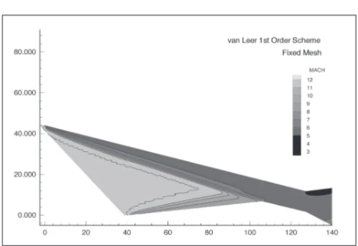
The results considering an inlet entrance Mach number
M∞ = 12 are discussed in detail in the paper. The Mach
contours obtained with the ive schemes are presented in Figs. 5–9 for the calculations with the coarse ixed mesh. The igures present, respectively, the results with
the centered scheme, the 1st- and 2nd-order van Leer
lux-vector splitting schemes and the 1st- and 2nd-order
Liou AUSM+ schemes. The contours indicate that the
overall low features are well captured by all solutions,
at least in the upstream portion of the inlet. However,
they also suggest that, at least with this coarse ixed
mesh, all schemes produce oscillations in the solution. The oscillations are more evident in the results with the centered scheme, as one might expect. Nevertheless, the somewhat ragged contours for the both upper and lower wall entrance shocks for all calculations are an indication that there are oscillations in these solutions. Moreover, the Mach number contours shown in Figs. 5–9 also indicate
that the resolution of low features downstream of the
interaction region of the two entrance shocks is not very good with this coarse mesh. Essentially, one cannot see
much of the shock relections and expansions that should
be present in these downstream regions.
A summary of the analysis of these igures indicates that the entrance low features are well captured by the
centered scheme, as already discussed, except that one can clearly see the oscillations upstream of the strong upper wall entrance shock. One can see in Figs. 6 and 8 that the 1st-order van Leer and 1st-order Liou schemes
smooth out the spatial gradients by the intrinsic artiicial
dissipation present in these schemes, which is typical of 1st-order upwind discretizations. Moreover, the 2nd-order schemes implemented in this work presented a better shock-capturing capability compared with the other schemes. They do not have as much shock-smearing as their 1st-order versions and, at the same time, they do not present as much evidence of solution oscillation as the 2nd-order centered scheme. Unfortunately, as discussions
Figure 4: Complete view of the three computational meshes
used in the present comparisons: (a) coarse ixed mesh; (b) ine ixed mesh; and (c) adaptive mesh.
Figure 5: Mach number contours obtained with the coarse
later in this paper will show, only the analysis of the Mach number contours can be misleading as far as an overall study of solution oscillations is concerned.
Corresponding results for the ine ixed grid are shown
in Figs. 10–14. These again consider an entrance
Mach number M∞ = 12 and calculations with the ive
discretization schemes are represented in these igures. The irst aspect which is clearly evident from the igures is that the upstream entrance shocks are much better deined in the iner grid solution. Moreover, some of the downstream low features, which could not be seen in the coarse grid solution, are now starting to become apparent in the ine
grid. However, the grid resolution in the downstream
portions of the low is clearly still not suficient to resolve all details of the lowield in these regions, especially for
the more dissipative 1st-order schemes.
The oscillations in the upper wall entrance shock for the
centered scheme solution are also quite visible in this ine ixed grid solution, as shown in Fig. 10. These oscillations are restricted to a narrower region of the low, as one should expect due to the increased mesh reinement, but they are
still present in the solution. Moreover, oscillations in the lower wall entrance shock can also be seen in Fig. 10. The
deinition of the entrance shocks in the upwind solutions is
improved with the current grid, both for the 1st- and the 2nd-order schemes. This improvement is consistent with the one observed for the centered scheme case. However, one can
observe some sort of an inlection in the upper wall entrance shock for the 2nd-order van Leer lux-vector splitting
scheme solution (see Fig. 12), which clearly does not have any physical meaning. Actually, it is possible to see a similar problem in the coarse grid solution with this scheme, shown in Fig. 7. The problem, however, becomes even more evident
in the ine grid result shown in Fig. 12. A close inspection
of the Mach number contours obtained with the 2nd-order AUSM+ scheme also reveals a similar inlection problem in the upper wall entrance shock. As one can see in Fig. 14, however, this spurious behavior is much less pronounced in the solution with the 2nd-order Liou scheme.
Despite the clear improvement in low feature resolution provided by the iner ixed mesh, as already pointed out,
an overall assessment of the previous results indicates that
some aspects of the low are still very poorly resolved even with this ine grid. In particular, one can observe
that the lower wall entrance shock is quite smeared
and that the downstream portions of the low are not
adequately resolved. Hence, the use of an adaptively
reined mesh seemed to be the best approach in order to
allow the grid density to be driven by the solution itself. The corresponding Mach number contours for freestream
Mach number M∞ = 12, computed with the inal adaptively
reined mesh, are shown in Figs. 15–19. In general, these results indicate a much sharper deinition of both upper and lower wall entrance shocks and of the low features
downstream of the shock interaction region. Although the full resolution of this interaction may still require further
grid reinement, the results in Figs. 15–19 can already provide an idea of the low structure in the downstream portions of the coniguration.
Figure 6: Mach number contours obtained with the coarse ixed
mesh for the 1st-order van Leer scheme (M∞ = 12).
Figure 7: Mach number contours obtained with the coarse ixed
mesh for the 2nd-order van Leer scheme (M∞ = 12).
Figure 8: Mach number contours obtained with the coarse ixed
Figure 9: Mach number contours obtained with the coarse ixed
mesh for the 2nd-order Liou scheme (M∞ = 12).
Figure 10: Mach number contours obtained with the ine ixed
mesh for the centered scheme (M∞ = 12).
Figure 11: Mach number contours obtained with the ine ixed
mesh for the 1st-order van Leer scheme (M∞ = 12).
Figure 13: Mach number contours obtained with the ine ixed
mesh for the 1st-order Liou scheme (M∞ = 12).
Figure 12: Mach number contours obtained with the ine ixed
mesh for the 2nd-order van Leer scheme (M∞ = 12).
Figure 14: Mach number contours obtained with the ine ixed
mesh for the 2nd-order Liou scheme (M∞ = 12).
One can see in Fig. 15 that the centered scheme still exhibits oscillations in this case, especially near the upper wall inlet lip. However, a comparison of Figs. 4 and 15 indicates that the oscillations mostly occur in a region in which the mesh is quite coarse, i.e., they are in
a region upstream of the densely reined mesh area due
to the presence of the upper wall shock. In any event,
with both 1st- and 2nd-order versions of the van Leer scheme, shown in Figs. 16 and 17, present a rather ragged
irst contour in the entrance shock region. Moreover, both
calculations also present considerable smearing of the weaker lower wall shock. Although, it is true that even this
shock is much better deined by the adaptively reined grid
solution with the two versions of van Leer’s scheme than corresponding results with the other grids. The solutions with the van Leer schemes do not show much detail of
the downstream portions of the low. Again, one can see
differences between the 1st- and 2nd-order results in this downstream region, but the scheme is clearly too diffusive
despite the strong mesh reinement in the region.
An analysis based solely on the Mach number contours in Figs. 15–19 would indicate that the calculations with both
versions of the AUSM+ scheme yield the best resolution
of low features in this case. Furthermore, the 2nd-order results in Fig. 19 provide the best deinition of both
upper and lower wall entrance shocks, of the result of the shock-shock interaction and of the downstream expansion
and compression regions. There are still indications of solution oscillations even for these results, especially near the upper wall inlet lip. However, they clearly provide
the best overall description of the low features among all
schemes and different meshes analyzed. Unfortunately, as the forthcoming discussion will show, there are also serious problems with the Liou scheme solutions, both for the 1st- and 2nd-order versions of the scheme, which complicate the selection of a best overall result among the various tests performed.
Dimensionless pressure distributions along both the inlet upper and lower walls were also analyzed in order to obtain a better assessment of the solution quality for all test cases. As before, all cases consider an entrance
Mach number M∞ = 12. An initial comparison shows
plots of pressure distributions, obtained with each one of the spatial discretization schemes studied, for all three meshes. The analytical solution for the inlet entrance
region is also shown in each igure. This solution is
correct up to the point in which structures resulting from
Figure 15: Mach number contours obtained with the adaptively
reined mesh for the centered scheme (M∞ = 12).
Figure 16: Mach number contours obtained with the
adap-tively reined mesh for the 1st-order van Leer
scheme (M∞ = 12).
Figure 17: Mach number contours obtained with the
adaptive-ly reined mesh for the 2nd-order van Leer scheme
(M∞ = 12).
Figure 18: Mach number contours obtained with the
adap-tively reined mesh for the 1st-order Liou scheme
the shock-shock interaction start to impinge upon the inlet walls. Hence, Fig. 20 presents the dimensionless wall pressure distributions, for both upper and lower walls, obtained with the centered scheme. All calculations eventually reach the correct post-shock pressure plateaux, for both upper and lower walls. However, the numerical solutions approach their corresponding plateaux rather slowly, or over a fairly long longitudinal distance, and in
a very oscillatory fashion for both ixed mesh solutions.
The behavior of the pressure distribution obtained with the adaptive mesh is far less oscillatory. The curve for the
coarse ixed mesh also presents a very distinctive pressure
peak immediately upstream of the expansion corner in the upper wall. This is caused by a shock, resulting from the shock-shock interaction, which impinges upon the upper wall. This shock, however, cannot be seen in the Mach
number contours shown in Fig. 5. In general, the results with the ine ixed grid and with the adaptive grid are
similar for this case, except for the oscillations in the upper
wall shock in the ixed grid solution, as already discussed.
The comparison of the results obtained with the two versions of the van Leer scheme is shown in Figs. 21 and 22, respectively for the 1st- and 2nd-order schemes. The pressure distributions in the upper wall shock are much less oscillatory in this case, especially for the 1st-order scheme solution. This is to be expected since this scheme is quite a bit more diffusive than the others tested here. Actually, the previous discussion has indicated that the van Leer scheme is more diffusive and, clearly, its 1st-order implementation is more diffusive than the 2nd-order one. The solution with the 2nd-order scheme again presents
oscillations in this region of the low for the coarse ixed
grid. Aside from the problems already discussed in the previous case with regard to the entrance shocks, one can also observe that there are marked differences in the pressure distributions, obtained with the different meshes,
in the downstream portion of the low. This is true for
both 1st- and 2nd-order cases, but it seems to be more pronounced in the 1st-order results. Moreover, the results with the 2nd-order version of the scheme are indicating a gentle oscillation in the upper wall pressure distributions
at x ≅ 70 cm. This feature can be seen in the results for
all three meshes with the 2nd-order van Leer scheme, although its spatial position is slightly different depending on the grid. Such oscillation is clearly incorrect, since the pressure must be constant in this region.
The results with the 1st-order and the 2nd-order Liou schemes are shown in Figs. 23 and 24. The most distinctive feature of these results is that, in both cases, the solutions have strong oscillations at the upper wall entrance shock. There are oscillations in the lower wall shock too, but these are mild compared with the ones
observed in the upper wall case. It is interesting that the
same extreme oscillations are observed both in the 1st-order results as well as in the 2nd-1st-order ones. The adaptive grid calculations present the results with the smallest oscillations in this case. However, even such milder oscillations would still be considered unacceptable if the
present low solver capability were to be coupled to the
equations describing the real gas effects present in practice for such applications. One can also observe that there is good agreement among the pressure distributions, obtained with the different meshes in this case, for the downstream
portions of the low. The agreement is not as good for the case of the coarse ixed mesh, but this mesh is too coarse to resolve low features in the downstream region anyway, as
already discussed. Moreover, Figs. 23 and 24 are showing pressure distributions in the downstream portions of the
low which are quite different from the ones obtained with
the van Leer scheme (see Figs. 21 and 22).
Further analysis of the results can be accomplished by looking at essentially the same data shown in Figs. 20 to 24, but from a different perspective. Therefore, Figs. 25–
Figure 19: Mach number contours obtained with the adaptively
reined mesh for the 2nd-order Liou scheme (M∞ = 12).
28 allow for a more direct comparison of the discretization scheme effects on the solution, for a given mesh. As before, the dimensionless pressure distributions along the upper and lower inlet walls are being shown in these
igures. The analytical solution for the pressure distribution
Figure 23: Analysis of the mesh effect in the wall pressure dis-tributions obtained with the 1st-order Liou scheme (M∞ = 12).
Figure 24: Analysis of the mesh effect in the wall pressure dis-tributions obtained with the 2nd-order Liou scheme (M∞ = 12).
Figure 25: Analysis of the discretization scheme effect in the wall pressure distributions obtained for the
adaptively reined grid (M∞ = 12). Comparison of
centered and 1st-order upwind schemes.
Figure 26: Analysis of the discretization scheme effect in the wall pressure distributions obtained for the
adaptively reined grid (M∞ = 12). Comparison of
centered and 2nd-order upwind schemes. Figure 21: Analysis of the mesh effect in the wall pressure
distributions obtained with the 1st-order van Leer scheme (M∞ = 12).
Figure 22: Analysis of the mesh effect in the wall pressure distributions obtained with the 2nd-order van Leer scheme (M∞ = 12).
along the upstream portion of both upper and lower inlet entrance walls is also shown for comparison purposes. The comparison in Fig. 25 includes the centered scheme and the two 1st-order upwind schemes, for solutions computed
comparison including the two 2nd-order upwind schemes is presented in Fig. 26. Aside from some aspects which have already been discussed, such as the fact that the Liou scheme solutions are very oscillatory at the entrance shocks, one can state that, in general, there is a fairly good correlation between the results with the centered scheme
and those with the AUSM+ scheme. This is true for both
1st- and 2nd-order implementations of the Liou scheme.
On the other hand, the results with the van Leer scheme are quite different from the others downstream of the expansion corners on both upper and lower walls. Although these differences are also present in the 2nd-order van Leer solutions, the discrepancies are more evident in the 1st-order results. Essentially, the solution for the 1st-order implementation of the van Leer scheme seems to indicate that shock waves impinge on the upper and lower inlet walls approximately at the location of the wall expansion corners. For the lower wall, it would be more precise to state that the impingement would occur at the upstream expansion corner. The results with the other schemes do not corroborate this observation. They show
no shock impingement at the inlet upper wall. In this case,
even the 2nd-order van Leer solution does not show any shock impingement on the upper wall. Moreover, for the lower wall, both 1st- and 2nd-order van Leer solutions are fairly similar and, again, they are completely different from the wall pressure distributions obtained with the other
schemes in this downstream low region. Nevertheless,
the wall pressure distributions obtained with the van Leer method indicate that this scheme is the most successful in preventing oscillations, among the algorithms tested, across the strong upper wall entrance shock. This is particularly true for the 1st-order version of the scheme.
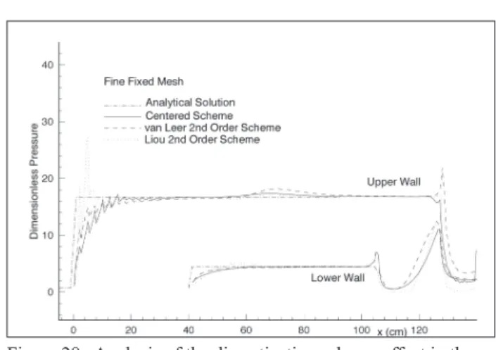
A similar comparison is shown in Figs. 27 and 28 for the
calculations performed with the ine ixed grid. The more
relevant comments which can be made in this case are essentially equivalent to those already discussed in the
context of the analysis of Figs. 25 and 26. In any event,
it is interesting to observe that the pressure distributions obtained with the van Leer scheme are very similar to those calculated by the other schemes in this case, especially for the 2nd-order version of the method. The 1st-order van Leer results, particularly for the upper wall, are still quite different from the pressure distributions obtained with the other schemes. Unfortunately, the better correlation
observed with the ine ixed grid can simply be the result
of having a mesh which is too coarse in the downstream
regions of the low to actually capture the phenomena that
should be present there.
Finally, pressure contours obtained with the adaptively
reined mesh are shown in Figs. 29–31. These igures
present, respectively, the contours for the solutions with the centered scheme, the 1st-order Liou scheme and the 2nd-order Liou scheme. The major objective of including
these igures here is to provide further understanding of the low features especially in the downstream regions.
The pressure contours seem to be more revealing for the
low structures which appear downstream of the shock-shock interaction region. In general, the three solutions
are quite similar in this case, as the previous discussions have already indicated. The more diffusive character of the 1st-order scheme is not as evident in Fig. 30, except for the thicker upper wall entrance shock. Pressure contours
calculated with the ixed meshes (not shown here) would
indicate that the additional numerical diffusivity of the 1st-order scheme would destroy some of the information in the downstream region. Moreover, it is also clear that the
upper wall entrance shock is more sharply deined by the
2nd-order upwind solution than by either the centered or
the 1st-order upwind calculations. The igures also seem to indicate that further reinement of the interaction region
Figure 27: Analysis of the discretization scheme effect in the
wall pressure distributions obtained for the ine
ixed grid (M∞ = 12). Comparison of centered and
1st-order upwind schemes.
Figure 28: Analysis of the discretization scheme effect in the
wall pressure distributions obtained for the ine
ixed grid (M∞ = 12). Comparison of centered and
would still be necessary in order to fully characterize these downstream structures.
It is important to emphasize that similar calculations were
performed for inlet entrance Mach numbers M∞ = 4, 8
and 16, in the context of the present study. These results
Figure 29: Dimensionless pressure contours obtained with the
adaptively reined mesh for the centered scheme
(M∞ = 12).
Figure 30: Dimensionless pressure contours obtained with
the adaptively reined mesh for the 1st-order Liou
scheme (M∞ = 12).
Figure 31: Dimensionless pressure contours obtained with
the adaptively reined mesh for the 2nd-order Liou
scheme (M∞ = 12).
are not included here because the conclusions that can be drawn are essentially equivalent to those obtained with
the M∞ = 12 solution. As one could clearly expect, the
oscillations observed in essentially all calculations here reported decrease as the inlet entrance Mach number is
lowered. In a similar fashion, results for the M∞ = 16 case are even more oscillatory than those here discussed.
Moreover, the authors would also like to emphasize that each case could be directly run with the adaptive
reinement capability. This was not done in the present work because the inal meshes, that would be obtained in such case, would be different since there are small differences in the converged solutions obtained with the various schemes. Therefore, the authors have chosen to compare the solutions obtained in a single mesh
generated by an adaptive reinement procedure using
one of the available spatial discretization schemes. Moreover, the most relevant comparisons in the present
case must be those between the adaptively reined mesh
results and the ones obtained with the ine ixed mesh,
because these two meshes have approximately the same number of control volumes. As the results presented in the paper have demonstrated, the quality of the solutions obtained with the adaptive grid is certainly better, for the same computational cost.
Furthermore, it is also important to emphasize that, in
actual light, an inlet low with entrance Mach number
equal to 12, or 16, could not be simulated with the perfect
gas assumption. In other words, real gas behavior would
have to be taken into account. From a physical standpoint, however, the present calculations could be considered as
the simulation of the cold gas lows which are usually achieved in experimental facilities such as gun tunnels. In order to extrapolate these results to actual light conditions,
dissociation and vibrational relaxation would certainly have to be included in the formulation. Nevertheless, the present simulations could be seen as a necessary step in the construction of a robust code to deal with the complete
environment encountered in actual light.
CONCLUDING REMARKS
The present work performed a comparison of ive different spatial discretization schemes for cold gas hypersonic low
simulations. The schemes presented here were applied to the
solution of supersonic and hypersonic inlet lows. The inlet
entrance conditions were varied from M∞ = 4 up to M∞ = 16.
An inviscid formulation was used and the luid was treated as a perfect gas. Clearly, for actual light condition simulation,
real gas effects would have to be taken into account. Here, however, the consideration of very high Mach number
lows simply has the objective of testing the behavior of the
The governing equations are discretized in an
unstructured triangular mesh by a cell-centered inite
volume algorithm. An edge-based data structure is used to store the connectivity information and this has yielded
an eficient procedure for interface lux calculations. The
equations are advanced in time by an explicit, 5-stage, 2nd-order accurate, Runge-Kutta time stepping procedure. The spatial discretization considers a 2nd-oder centered scheme and two upwind schemes, namely a van Leer and
a Liou lux-vector splitting scheme, with both 1st- and
2nd-order implementations. The authors believe that the form in which the Liou scheme has been implemented in the present unstructured grid context represents an original contribution, since the splitting is performed in a direction normal to the triangular cell edges. Therefore, instead of
having to compute x and y splittings for a 2-D low, only
one single splitting calculation is performed per cell edge in the edge-normal direction.
The implementation of the 2nd-order versions of the two upwind schemes uses MUSCL reconstruction in order to obtain left and right states at interfaces. An original procedure for performing this reconstruction is
presented which deines a 1-D stencil in the edge-normal
direction and, therefore, obviates the need to compute
low property gradients at each cell. This 1-D stencil is
constructed by identifying an additional triangle along the edge-normal direction which is used for the linear reconstruction process. All search operations necessary
for this identiication are performed at a pre-processing stage, yielding a very eficient algorithm. Moreover, the
2nd-order versions of the upwind schemes require the implementation of limiters in order to try to minimize oscillations at discontinuities. A few different limiters were actually coded, but only results with the minmod limiter were reported here. Previous experience with the other limiters has indicated that most of them fail to converge to machine zero, whereas the minmod limiter typically reaches machine zero for the cases analyzed here.
Results with unstructured ixed meshes, both coarse and ine, were obtained and compared with those calculated with an appropriate adaptively reined mesh. The various
calculations indicate that it is possible to obtain converged solutions with centered schemes, even for the very high
Mach number lows considered in the present work.
However, these solutions will most certainly be oscillatory. Moreover, the solutions with both 1st- and 2nd-order versions of the Liou scheme are also quite oscillatory, especially across the strong upper wall entrance shock.
The use of adaptively reined meshes has contributed to
reduce the oscillations in all cases. On the other hand, this has not been enough to completely remove the oscillations in the cases in which they appear. The 1st-order van Leer
lux vector splitting scheme has drastically reduced the
low property oscillations. However, as one could expect,
this 1st-order method also causes considerable smearing of
the low discontinuities due to the excessive intrinsically added artiicial dissipation.
Among the various schemes implemented, the
2nd-order AUSM+ method has provided the sharpest shock
deinitions. This is true both with ixed and with adaptively reined meshes. However, even with the adaptively reined
mesh, the 2nd-order Liou scheme has shown overshoots in the pressure distributions at the upper wall entrance shock.
The situation is a lot worse for the ixed mesh solutions
with this scheme. Moreover, one must also observe that both 2nd-order upwind methods have a slower convergence rate than the other schemes implemented. Furthermore, for the higher Mach number cases, the 2nd-order implementation of the Liou scheme was not able to reach machine zero, even with the minmod limiter.
The mesh adaptation procedure implemented was able to generate good quality meshes for the cases considered
in the present work. The adaptation strategy identiied
the more relevant high gradient areas and provided an adequate grid point clustering in the important regions. Moreover, some simple mesh smoothing procedures have also been implemented, through point movement and diagonal swapping techniques, which contributed
to the high quality of the meshes after reinement. It is
also important to emphasize that the tests conducted in the context of the present work have only used a sensor
based on low density gradients. Although this has
produced good results for the present cases, one can conceivably argue that there are other important cases in which this approach would not be the most appropriate. Therefore, further testing would clearly be necessary in order to achieve a more robust strategy for the sensor
deinition.
ACKNOWLEDGMENTS
The authors gratefully acknowledge the partial support for this research provided by Conselho Nacional de Desen-
volvimento Cientíico e Tecnológico, CNPq, under the
Integrated Project Research Grant No. 312064/2006-3.
This work is also supported by Fundação de Amparo à Pesquisa do Estado de São Paulo, FAPESP, through
Process No. 2004/16064-9.
REFERENCES
Anderson, W. K., Thomas, J. L., Van Leer, B., 1986, “A Comparison of Finite Volume Flux Vector Splittings for
Azevedo, J. L. F., 1992, “On the Development of Unstructured Grid Finite Volume Solvers for High Speed
Flows”, IAE, São José dos Campos, Brazil, (Report
NT-075-ASE-N/92).
Azevedo, J. L. F., Figueira da Silva, L.F., 1997, “The Development of an Unstructured Grid Solver for Reactive
Compressible Flow Applications”, 33rd AIAA/ASME/
SAE/ASEE Joint Propulsion Conference & Exhibit,
Seattle, WA (AIAA Paper 97-3239).
Azevedo, J. L. F., Oliveira, L. C., 1994, “Unsteady Airfoil Flow Simulations Using the Euler Equations”,
Proceedings of the 12th AIAA Applied Aerodynamics
Conference, Part 2, Colorado Springs, CO, pp. 650-660,
(AIAA Paper 94-1892-CP).
Hirsch, C., 1990, “Numerical Computation of Internal
and External Flows”, Vol. 2: Computational Methods for
Inviscid and Viscous Flows, Wiley, New York, Chap. 20,
pp. 408-443.
Jameson, A., Mavriplis, D., 1986, “Finite Volume Solution of the Two-Dimensional Euler Equations on a Regular
Triangular Mesh”, AIAA Journal, Vol. 24, No. 4, pp. 611-618.
Jameson, A., Schmidt, W., Turkel, E., 1981, “Numerical Solution of the Euler Equations by Finite Volume Methods
Using Runge-Kutta Time-Stepping Schemes”, AIAA 14th
Fluid and Plasma Dynamics Conference, Palo Alto, CA
(AIAA Paper 81-1259).
Liou, M.S., 1994, “A Continuing Search for a Near-Perfect
Numerical Flux Scheme. Part I:AUSM+ ”, NASA Lewis Research Center, Cleveland, OH (NASA TM-106524).
Liou, M.S.,1996,“A Sequel to AUSM: AUSM+”, Journal
of Computational Physics, Vol. 129, pp. 364-382.
Lyra, P. R. M., 1994, “Unstructured Grid Adaptive Algorithms for Fluid Dynamics and Heat Conduction”, Ph.D.Thesis, Department of Civil Engineering, University of Wales Swansea, Swansea, Wales, U.K.
Mavriplis, D.J., 1988, “Multigrid Solution of the Two-Dimensional Euler Equations on Unstructured Triangular
Meshes”, AIAA Journal, Vol. 26, No.7, pp. 824-831.
Mavriplis, D.J., 1990, “Accurate Multigrid Solution of the Euler Equations on Unstructured and Adaptive Meshes”,
AIAA Journal, Vol. 28, No. 2, pp. 213-221.
Pulliam, T. H., 1986, “Artiicial Dissipation Models for the Euler Equations”, AIAA Journal, Vol. 24, No. 12, pp.1931-1940.
Steger, J. L., Warming, R. F., 1981, “Flux Vector Splitting
of the Inviscid Gasdynamic Equations with Application
to Finite-Difference Methods”, Journal of Computational
Physics, Vol. 40, No. 2, pp. 263-293.
Van Leer, B., 1979, “Towards the Ultimate Conservative Difference Scheme. V. A Second-Order Sequel to Godunov’s Method”, Journal of Computational Physics,
Vol. 32, No. 1, pp. 101-136.
Van Leer, B., 1982, “Flux-Vector Splitting for the
Euler Equations,” Proceedings of the 8th International