Alberto W. S. Mello Jr* Institute of Aeronautics and Space São José dos Campos - Brazil [email protected]
Daniel Ferreira V. Mattos Institute of Aeronautics and Space São José dos Campos - Brazil [email protected]
* author for correspondence
Reliability prediction for
structures under cyclic loads and
recurring inspections
Abstract: This work presents a methodology for determining the reliability of fracture control plans for structures subjected to cyclic loads. It considers the variability of the parameters involved in the problem, such as initial law and crack growth curve. The probability of detection (POD) curve of the ield non-destructive inspection method and the condition/environment are used as important factors for structural conidence. According to classical damage tolerance analysis (DTA), inspection intervals are based on detectable crack size and crack growth rate. However, all variables have uncertainties, which makes the inal result totally stochastic. The material properties, light loads, engineering tools and even the reliability of inspection methods are subject to uncertainties which can affect signiicantly the inal maintenance schedule. The present methodology incorporates all the uncertainties in a simulation process, such as Monte Carlo, and establishes a relationship between the reliability of the overall maintenance program and the proposed inspection interval, forming a “cascade” chart. Due to the scatter, it also deines the conidence level of the “acceptable” risk. As an example, the damage tolerance analysis (DTA) results are presented for the upper cockpit longeron splice bolt of the BAF upgraded F-5EM. In this case, two possibilities of inspection intervals were found: one that can be characterized as remote risk, with a probability of failure (integrity nonsuccess) of 1 in 10 million, per light hour; and other as extremely improbable, with a probability of nonsuccess of 1 in 1 billion, per light hour, according to aviation standards. These two results are compared with the classical military airplane damage tolerance requirements.
Keywords: Reliability, Structure integrity, Fatigue, Damage tolerance.
LIST OF SYMBOLS AND ABBREVIATION
a Crack size
a Parameter of the POD curve
a0 Crack length for zero-detection probability
COV Coeficient of Variation
CDF Cumulative distribution function DTA Damage tolerance analysis FCL Fatigue critical location
l Parameter of the POD curve NDI Non-destructive inspection POD, Pd Probability of Detection PDF Probability distribution function
s, s(t) Standard deviation, Standard deviation as function of time
INTRODUCTION
Structures such as airplanes, bridges, ships, etc, are subjected to cyclical loads that can lead any initial crack
to a catastrophic failure. Ideally, any fracture control plan should be based upon the acceptable probability of failure.
The crack propagation rate, the ield inspection, and the
quality of the material are subject to uncertainties that
make a deterministic reliability study for the case dificult
(Provan, 2006). Many of the parameters and variables used in fracture control have a scatter factor that must be accounted for in life prediction. All material properties have variability. In most cases, the structural loads are statistical variables. Crack detection capability is also governed by statistics. There is a non-zero probability that a crack will be missed, in spite of the sophisticated inspection method to be used. For this reason, in a crack growth curve, a scatter factor has always to be considered to determine the inspection intervals. The scatter factor depends on the accuracy of the data used as well as the
speciication that must be satisied.
Primary components are inspected upon manufacture and undergo an extremely strict quality control system. For
each component, it can be assured that if a law exists
it is smaller than a guaranteed size - ag. This guaranteed
Received: 18/09/09 Accepted: 28/10/09
Every time the structure is inspected there is a probability of missing the crack, regardless of its size. Naturally, the inspection may be performed several times during the structure service life, which will increase its probability of detection.
On the other hand, the size of the crack at a certain service
life time depends not only upon the initial law size but
also the crack growth rate. There is uncertainty about how fast the crack grows, which can be visualized in Figure 3.
Figure 1: CDF for initial crack size.
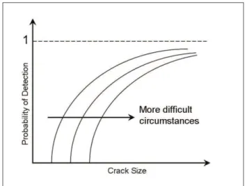
Figure 2: Crack Probability of Detection Curves.
Figure 3: Scatter in Crack Growth Curve.
maximum law depends upon the type of inspection
(Broek, 1989; Knorr, 1974; Lewis, 1978).
On the other hand, each component is assumed to have a law
of at least a1, which represents the minimum intergranular “defect” and/or machining surface imperfection present in the material (Gallagher, 1984).
The initial law size can be considered as a uniform
distribution between a1 and ag (Knorr, 1974), as depicted in Figure 1.
From the moment of manufacture, the structure has to be
inspected by a speciied NDI (non-destructive inspection)
method. The probability of detection for each method depends upon the crack size and the accessibility of the inspected location, as show in Figure 2.
The point where the curves cross the horizontal axis is the zero probability of detection and is dictated by the
resolution of the NDI equipment under that speciic
condition (Lewis, 1978).
The crack size for each operation time and for a prescribed initial crack follows a normal distribution with the average of a predicted crack growth curve with
a given coeficient of variation (Broek, 1989). Figure 3
shows typical crack growth curves with a possible scatter in the crack growth rate.
In order to obtain the reliability of a structure submitted to
cyclic loads, all these uncertainties must be quantiied and
accounted for. The following Section will describe each of the uncertainties involved in the analysis and how they can be anticipated.
UNCERTAINTIES
Initial Crack Size
Each structure is made of components that had to be machined and assembled to form the whole part. The machining process as well as the assembly can introduce small damage to the components that can lead to propagating cracks (Knorr, 1974). Also, even for very well controlled processes, there is an
intrinsic “crack”, which can be deined as imperfections in the
grain boundary of the metal (ASM Handbook, 1992). Figure 4 illustrates how this imperfection may occur in the grain boundary level.
As a consensus, it has been usual to consider a value of
However, any number can be speciied, according to the
requirements. This is the a1 parameter exempliied in Figure 1.
in Figure 6. This Figure depicts how this scatter can be understood, by showing a normal distributed crack growth rate with a central value, which is the average curve predicted by fracture mechanics, and its standard
deviation. A coeficient of variation between 10 and 20
per cent normally covers all the uncertainties related to the crack growth rate (Broek, 1989).
Figure 4: Initial law formed in the grain boundary
On the other hand, before being assembled to form the structure, all components are inspected by the manufacturer, by means of a suitable non-destructive inspection method. So that, for each component, or complete structure, there is a guarantee that if any imperfection exists it is smaller than in-Lab detection size. Normally, this guaranteed value is in the order of 1.27 mm (0.05”). This is the ag parameter illustrated in Figure 1 (Knorr, 1974).
Crack Growth Curve
All material properties, including toughness, show variability. According to MIL-A-8866 (USAF, 1974), in most cases the structural loads are statistical variables. The pressure vessel may be well controlled, but random
luctuations may occur. Loads on bridges vary widely depending upon trafic; they can be estimated but cannot
be known until after the fact. Despite the state-of-the-art in measuring loads, fatigue life prediction is based on the assumption that previous measured loads will be repeated in the future. In addition, there are errors due to shortcomings and limitations of the analysis, due to the limited accuracy of loads and stress history, and due to simplifying assumptions. For the effects of all these assumptions, it is preferable to use best estimates and
average data and to apply the variability on the inal crack
growth curve.
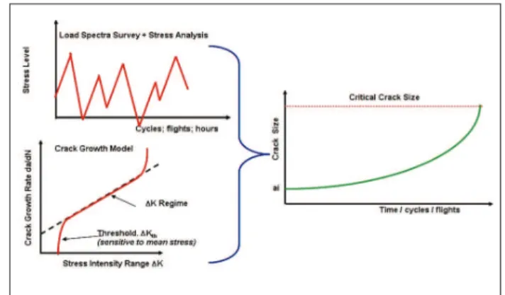
So that, with the best information from the load history and material properties, by using the fracture mechanics approach, an average crack growth curve can be obtained, as depicted in Figure 5.
To summarize all the uncertainties of loads and material properties in the crack growth curve, a scatter can be applied, with the mean value on the predicted curve and with a given distribution from that value, as shown
Figure 5: Crack growth curve from the best known opera-tional and material data.
Figure 6: Scatter applied on average crack growth curve.
NDI Probability of Detection
As already discussed, crack detection is governed by statistics. There is a non-zero probability that a crack will be missed, despite the sophisticated inspection methodology.
This work focuses on the available data from the following NDI techniques: Eddy current, ultrasound, dye penetrant, x-ray and visual. It is not the scope of this work to discuss how the inspections are performed. None of the inspection processes will be discussed. If in the future an NDI technique is improved, the parameters presented in this work can be supplemented and the overall reliability determination tool will still be valid.
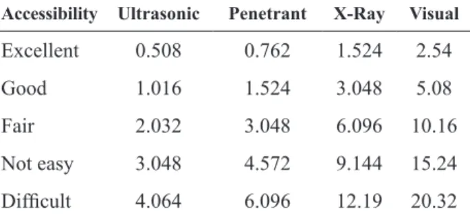
a0 is function of the inspection method and the accessibility of the area to be inspected (Table 2).
Table 1: l/a0 for different inspection methods (Knorr, 1974; Lewis, 1979)
Method l/ a0
Ultrasonic 3.00 Dye Penetrant 2.17 Eddy-current 2.23
X-ray 2.50
Visual 2.00
Table 2. a0, in millimeters, for various inspection methods and accessibilities (Knorr, 1974; Lewis, 1979).
Accessibility Ultrasonic Penetrant X-Ray Visual
Excellent 0.508 0.762 1.524 2.54 Good 1.016 1.524 3.048 5.08 Fair 2.032 3.048 6.096 10.16 Not easy 3.048 4.572 9.144 15.24
Dificult 4.064 6.096 12.19 20.32
METHODOLOGY
The proposed solution for the problem involves Monte Carlo simulation (Manuel, 2002). The process consists of generating random numbers for ai and crack growth curve rate, change the inspection interval and compute the probability of detection due to recurring inspections during the structure service life.
As a reinement of the method, the Latin Hypercube
procedure was also proposed (Manuel, 2002), where the simulation domain is divided into subdomains to better distribute the random numbers.
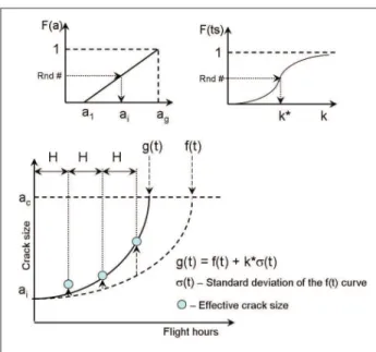
All variables in the problem are considered uncorrelated. The procedure for getting ai and the variability of the crack growth curve is summarized in Figure 7. In this Figure, the
distribution of initial law is considered to be uniform and the
crack growth rate is Gaussian. For every cycle of iteration,
the initial law size is randomly picked between a1 and ag,
and the effective crack size is computed on the curve g(t). Being f(t) the average crack size as function of the variable t
(cycles, time, lights etc.), g(t) is given by g(t) = f(t) + k*s(t). Where k* is the number of standard deviations obtained in
the N(0,1) curve by random generation. s(t) is the standard deviation expected for that crack size.
resolution of the eye, for ultrasonic inspection by the wave length, and so on. In the opposite direction, even for very large cracks, the probability of detection is never equal to 100 per cent, because any crack may be missed. Several
ield data on the reliability of non-destructive inspection
have shown that the probability curves have the general form shown in Figure 2, which can be described by the equation (Broek, 1989):
p = 1- e -{(a-a0)/(λ-a0)}α (1)
where a0 is the crack size for which detection is absolutely impossible (zero probability of detection), a and l are parameters determining the shape of the curve. It is important to distinguish between the detectable crack size and the constant a0 that appears in the equation. The detectable crack size ad is a general term whereas a0 represents a parameter in Equation 1. This equation gives the probability, p, that a crack of size a will be detected in one inspection by one inspector. The probability of non-detection is 1- p. A crack is subjected to inspection several times before it reaches the permissible size. At each inspection there is a chance that it will be missed. At successive inspections, the crack will be longer, and the probability of detection is higher, but there is still a chance that it may go undetected. The probability of detection is then:
p = 1 - ∏ (1 -n pi )
i=1
(2)
where pi is the probability of detection for each crack size, that follows a curve such as Figure 2, and n is the number of inspections.
The parameters a0, a and l were obtained from Knorr (1974) and Lewis (1978) and they are summarized here:
1 - For Eddy Current inspection method:
a0 = 0.889 mm (0.035”)
l = 1.98 mm (0.078”)
a = 1.78
2 - For all other inspection methods:
a = 0.5
By systematic variation in the inspection interval - H, the crack growth curve and the crack POD are updated to determine the cumulative probability of detection for the predicted structure life time. Figure 8 sketches one step of the process.
reliability. For example, if 99.9 per cent reliability is desired
with a 95 per cent conidence level, it is necessary that 95
per cent of the simulated cases for that particular reliability be at the right for the assumed inspection interval. Figure 10
depicts how the conidence level is considered. In this case, the
inspection interval H1 has a 99.9 per cent probability of going
through its service life intact, with 95 per cent conidence level.
Figure 7: Process of obtaining the crack size during each inspection.
Figure 8: One step of the overall process.
Repeating the procedure several times, a probability distribution region is expected, as shown in Figure 9. Therefore, the reliability of the overall structure remaining safe during its operational life can be predicted. Because for a given inspection interval there will always be scatter during the simulation, a cascade like chart is expected (Fig. 9). Hence, it is possible to establish a relationship between the probability of the structure being safe, given
an inspection interval, with a level of conidence.
The current work proposal is to determine the conidence
level by counting the number of points around the expected
Figure 9: Overall reliability as function of Inspection Interval.
The next Section describes the implementation of the proposed methodology in determining the reliability of structures subjected to cyclic loads under a fracture control maintenance plan.
Application Procedures
A dedicated computer program was developed to provide an automated engineering tool for recurring inspection
Figure 10: Inspection interval H1, given 99.9 per cent
reliability analysis. This program incorporates all the processes described here. The software main screen is as depicted in Figure 11.
inspection interval and how to randomize the variables. The minimum reliability is a saving time parameter that investigates probabilities of success above a given level. The random generation procedure may be divided in up to
100 partitions, for use of Latin Hypercube reinement. The
numbers are then randomized within each partition.
Figure 11: Main screen of the NDI Reliability Program
The irst step in the analysis is to load the crack growth curve. The data ile must be in tabulated text format. The irst column must contain the time (hours, cycles, lights
etc.) and the second column the crack size.
When crack growth data is uploaded, the program opens
another screen with the itted curve, as shown in Figure 12. The next steps are to deine which type of NDI will be performed in the ield and the accessibility location, the
boundaries for the initial crack and the type of distribution assumed for each of the uncertainties. This version of the program allows uniform distribution for ai and uniform or normal (Gaussian) distribution for the crack growth curve. Figure 13 shows the NDI setup screen.
Figure 12: Crack Growth Curve [8].
The options in the advanced menu (Fig. 14) are the minimum reliability level to be investigated, the maximum inspection interval to be considered, the increment in the
Figure 13: Program NDI setup screen.
The Analysis Menu option opens another screen allowing
simulation and deinition of the NDI interval, based on the
desired reliability.
For each type of inspection and/or access there is a better minimum probability to be chosen in the setup screen. For instance, for “Eddy Current” method, the POD curve approaches the curve for very small cracks. It means that despite the crack growth curve, one inspection in the life time will give a very high probability of detection. For
this case, the best result will be obtained by setting the minimum reliability to 0.99 or above.
The next Section discusses the results obtained for one of the fatigue critical locations from the damage tolerance analysis of the Brazilian Air Force upgraded F-5EM, performed according to the MIL-STD-1520C (USAF, 2005).
RESULTS
One F-5EM FCL, as presented by Mattos (2009), is the splice bolt in the upper cockpit longeron at Fuselage Station 284, as illustrated in Figure 15.
This is based on an initial law size of 2.74 mm (0.108”),
with a scatter factor of two.
This component will be inspected by dye penetrant technique. As the component is removed from the splice
area and taken to a laboratory, accessibility is classiied as excellent. The minimum law will be assumed to be
0.127 mm (0.005”) and the guaranteed value of maximum
crack size as new is 1.27 mm (0.05”). The coeficient of
variation (C.O.V) of the crack growth curve is given to be 10 per cent and it is normally distributed.
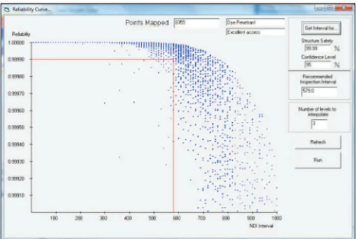
With all these parameters and starting the investigation at 99.9 per cent, the reliability chart is as shown in Figure 17. According to the MPH-830 (IFI, 2005), the characterization for improbable and extremely improbable is one in ten
million and one in one billion per light hour, respectively.
Figure 15: Upper longeron splice bolt F-5EM FCL @ FS 284 (Mello Jr., 2009).
This FCL has a crack curve as shown in Figure 16. This result is for the structure submitted to fatigue load spectrum
of the Canoas Air Force Base leet (Mello Jr., 2009).
Figure 16: Crack growth curve for the F-5EM upper cockpit longeron splice bolt (Data from Mello Jr., 2009).
According to the “Airplane damage tolerance requirements” (USAF, 1974) the suggested recurring
inspection interval for this component is 653 light hours.
Figure 17: Suggested light hour interval for a 0.01 per cent risk
in the structure life time, dye penetrant inspection.
The result presented in Figure 17 shows a suggested
interval of 579 light hours for a 0.01 per cent risk in the
structure life time. The procedures adopted in this work recommend dividing the risk by the suggested inspection
interval to obtain the estimated risk per light hour.
Therefore, for the determined recurring inspection time,
the risk is 0.0001/579 = 1.73 10-7 per light hour. This risk
falls within the improbable failure risk, as described in the MPH-830.
In order to investigate the extremely improbable risk, it is
necessary to reine the analysis. In this case, the starting
point must be 99.999 per cent. Figure 18 shows the reliability chart for this case.
The suggested inspection interval for a risk of 0.00001
per cent in a life time is 295 light hours. The risk per light hour may be estimated as 0.0000001/295 = 3.4 10-10,
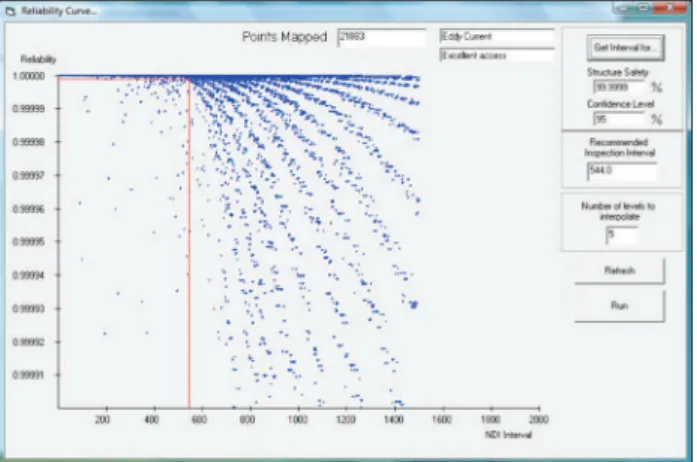
One suggestion that arises is the possibility of changing the NDI method. Figure 19 shows the result for an analysis aimed at the one in one billion probability of non success, but considering that the item would be inspected by eddy current. The result for that is the recommended inspection
interval of 544 light hours, for the extremely improbable
risk.
structure subjected to dynamic loads. An overview was presented of the parameters involved in the fracture control procedures, and a solution, using an automated code that could incorporate the uncertainties to determine
the reliability of the structure with a conidence level,
was proposed. Also, a description was given of how to determine each of the variables in the problem, considering variations for the NDI methods commonly used in the
ield, for recurring inspections.
The methodology used considers Monte Carlo simulation
with a reinement for Latin Hypercube technique. The
reliability curve is obtained by generation of random number for several inspection intervals. The chart
reliability vs. inspection interval can be mapped and the
safety probability can be obtained with a conidence level.
For the given examples, a structure, which is submitted to dye penetrant inspection, with excellent accessibility,
must be inspected every 579 light hours for an improbable risk of failure, at 95 per cent conidence level.
To categorize the risk as extremely improbable, recurring
inspections must be every 295 light hours. Following
the standards for military airplane damage tolerance analysis, the recommended inspection interval would
be 653 light hours. One alternative for increasing the
recurring inspection time, while keeping the risk very low, is to improve the NDI method. One example shows that by alternating the inspection from dye penetrant to eddy current, the extremely improbable risk interval would
increase from 295 to 544 light hours.
REFERENCES
ASM Handbook, 1992, “Failure analysis and prevention”, 9. ed., Materials Park, OH, (ASM International, vol. 11), pp.15-46.
Broek, D., 1989, “The practical use of fracture mechanics”. Galena, OH. Kluwer Academic, pp. 361-390.
Gallagher J. P., 1984, “USAF damage tolerant design handbook: Guidelines for the analysis and design of damage tolerant aircraft structures”, Dayton Research Institute, Dayton, OH, pp. 1.2.5-1.2.13.
IFI, 2005, “Análise e gerencialmento de riscos nos vôos de
certiicação”, MPH-830, Instituto de Fomento à Indústria. Divisão de Certiicação de Aviação Civil, São José dos
Campos, S.P., Brasil.
Knorr, E., 1974, “Reliability of the detection of laws and of the determination of law size”, AGARDograph,
Quebec, Nº. 176, pp. 398-412.
Figure 18: Suggested light hour interval for a 0.0001 per cent risk
in the structure life time, dye penetrant inspection.
Figure 19: Suggested light hour interval for a 0.0001 per cent
risk in the structure life time, eddy current inspection.
By way of observation, it is important to emphasize that many of the parameters and variables playing a role in fracture control sometimes vary beyond the expected values. The sole objective of this work is to provide an aid to fracture control measures so that cracks can be eliminated before they become dangerous, by either repair or replacement of the component. All the assumptions are hypotheses to allow predictions based on the best available tools.
CONCLUSION
Lewis W. H. et al., 1978, “Reliability of non-destructive inspection”, SA-ALC/MME. 76-6-38-1, San Antonio, TX.
Manuel, L., 2002, “CE 384S - Structural reliability course: Class notes”, Department of Civil Engineering, The University of Texas at Austin, Austin, TX.
Mattos, D. F. V. et al., 2009, “F-5M DTA Program”. Journal of Aerospace Technology and Management. Vol.1, Nº1, pp. 113-120.
Mello Jr, A.W.S. et al., 2009, “Geração do ciclo de tensões
para análise de fadiga, Software GCTAF F-5M”, RENG
ASA-I 04/09,IAE, São José dos Campos, S.P., Brasil.
Provan, J. W., 2006 ,“Fracture, fatigue and mechanical reliability: An introduction to mechanical reliability”, Department of Mechanical Engineering, University of Victoria, Victoria, B.C.
USAF., 1974, “Airplane damage tolerance requirements”.
Military Speciication. Washington, DC. (MIL-A-83444).
USAF., 1974, “Airplane strength and rigidity reliability requirements, repeated loads and fatigue”. Military
Speciication. Washington, DC. (MIL-A-008866).
![Figure 12: Crack Growth Curve [8].](https://thumb-eu.123doks.com/thumbv2/123dok_br/18888600.424429/6.918.463.814.548.864/figure-crack-growth-curve.webp)