This is an Open Access article distributed under the terms of the Creative Commons Attribution Non-Commercial License Received 14 Feb., 2017
Accepted 11 May, 2017
E-mails [email protected] (FMC), [email protected] (PRFT), [email protected] (DBA)
Abstract: The technique of weaving by magnetic arc deflection was developed a few years ago to enable the oscillation of the weld pool, thus, causing grain refinement and improving the properties on the welded joint. This paper aims to propose two heat source models that include effects of magnetic arc deflection on a bead-on-plate GTAW process in numerical simulations by using the finite element method. Two cases are studied. In the first case, non-deflected arc and straigth magnectic deflected arc along the torch movement are carried out and compared to numerical simulations. Temperatures at three different points on the backside of the plates (two away from the welding center line and one in its center) and weld pools of SAE 1020 3.2 mm and 6 mm thick steel plates are analyzed. Results obtained by numerical simulations are close to the experimental ones. In the second case, welding with weaving (frequency of 1Hz) on 3 mm thick steel plates is analyzed. The bead width and its visual presentation are compared to experimental results, which show good agreement with both proposed models.
Key-words: Heat source model; Numerical simulation; GTAW process; Magnetic arc deflection.
Dois Modelos de Fontes de Calor para a Simulação de Processos de
Soldagem com Delexão Magnética do Arco
Resumo: A técnica de tecimento por deflexão magnética do arco foi desenvolvida há alguns anos para permitir a oscilação da poça fundida, causando o refinamento de grão e melhorando as propriedades da junta soldada. Este artigo tem como objetivo propor dois modelos de fontes de calor que inclui os efeitos de deflexão magnética do arco em um processo GTAW sobre chapa nas simulações numéricas pelo uso do método dos elementos finitos. Dois casos são estudados. No primeiro, são comparadas as simulações numéricas para o arco sem deflexão e para o arco com deflexão magnética fixa ao longo do movimento da tocha. São analisadas as temperaturas em três pontos na parte inferior da chapa (dois afastados da linha de centro de soldagem e outro no centro) e poças de fusão para chapas de aço SAE 1020 e espessuras de 3,2 e 6 mm. Os resultados obtidos pelas simulações numéricas estão muito próximos aos experimentais. No segundo caso, é analisada a soldagem com tecimento (frequência de 1Hz) em chapas de aço de 3 mm de espessura. São comparadas as larguras do cordão e sua forma geométrica com os resultados experimentais, que mostram a boa concordância obtida pelos dois modelos propostos.
Palavras-chave: Modelo de fonte de calor; Simulação numérica; Processo GTAW; Deflexão magnética do arco.
1. Introduction
Welding with weaving is a widespread process in which the torch movement enables the deposit of wider weld bead with lower penetration. The weaving technique by magnetic arc deflection has recently been developed to enable the oscillation of the weld pool and, consequently, has caused grain refinement and has improved the properties on the welded joint. Experiments carried out by Sundaresan and Ram (1999) with titanium alloy showed that the magnetic deflection applied to TIG welding processes causes significant grain refinement. Similarly, Kumar et al. (2008) and Lim et al. (2013) also reported the increase
Two Heat Source Models to Simulate Welding Processes with Magnetic
Delection
Fernanda Mazuco Clain1, Paulo Roberto de Freitas Teixeira1, Douglas Bezerra de Araújo2
as those presented in magnetic weaving. Hongyuan et al. (2005), for example, developed a numerical model of heat input source applied to cases in which magnetic arc deflection is caused by the magnetic interaction in twin wire GMAW welding. In this numerical model, the magnetic arc deflection is caused by the torch inclination in relation to the welding plane by employing a double ellipsoid heat source model.
The aim of this study is to develop and validate two heat input source models by ANSYS Multiphysics software, which is FEM based model, to simulate the magnetic arc deflection in weld bead in autogean GTAW process. Both models are based on a Gaussian surface flux distribution, which has the advantage of having only two degrees of freedom (arc efficiency and radial distance from the center) and being suitable for a range of welding powers and plate thicknesses and diferent types of welding processes (Teixeira et al., 2014; Farias et al., 2017; Venkatkumar and Ravindran, 2016; Khurram et al., 2013; Hussain and Sherif El-Gizawy, 2016). Firstly, numerical simulations are compared with experimental ones for non-deflected arc to calibrate numerical models. Afterwards, straight magnetic deflected arcs along the torch movement are used for validating both models. In these experiments, fixed deflection of the arc along the welding is imposed to avoid a more complicated analysis if the torch weaves and, therefore, to enable the proposed models to be easily validated. Temperatures at three different points on the backside of the plates (two away from the welding center line and one in its center) and weld pools of SAE 1020 3.2 mm and 6 mm thick steel plates are analyzed. Finally, welding with weaving (frequency of 1Hz) on 3 mm thick steel plates is analyzed. Comparisons of width and visual presentation of the bead and experimental results (Larquer and Reis, 2016; Larquer et al., 2016) are carried out.
2. Materials and Methods
In order to simulate welding with magnetic deflection of the arc, a new heat source model is necessary. This new model can be developed by modifying existent models, as shown by Hongyuan et al. (2005). In this paper, two models are proposed, both based on the two-dimensional heat source model with Gaussian distribution, since this model has few degrees of freedom that allow quickly parameterization (Goldak et al., 1984).
To validate the proposed models, a first case is studied with magnetic deflection of the arc, but without weaving. Then, a second case is studied to validate the models for welding with weaving.
2.1. Governing equations and the Gaussian heat source model
The thermal field in welding processes is governed by the heat conduction equation. A phase change with melting and solidification is involved in the welding process. Enthalpy methods are some of several techniques to deal with this type of problem (Hu and Argyropoulos, 1996). The essential feature of basic enthalpy methods is that the evolution of the latent heat is accounted for the enthalpy as well as the relation between enthalpy and temperature. These methods are based on the heat conduction equation expressed in function of the enthalpy (H) as follows (Equation 1)
[ ( )]
( ) T ( ) T ( ) T H T
k T k T k T
x x y y z z t
∂ ∂ + ∂ ∂ + ∂ ∂ =∂
∂ ∂ ∂ ∂ ∂ ∂ ∂ (1)
where T is the temperature, k(T) is the thermal conducivity, ρ(T) is the speciic mass, Cp(T) is the speciic heat and
( ) p( )
H =
∫
ρ
T C T dT (2)The thermodynamic boundary conditions on the external surfaces of the solid comprise heat transfer for convection and radiation. The heat flow density for convection (q
c) in the environment gas or liquid is given by Newton’s heat transfer law (Equation 3):
0
(
)
c c
q
=
h T
−
T
(3)where T is the temperature of the external surface, T0 is the temperature of gas or liquid and hc is the coeicient
of convecive heat transfer. This coeicient depends on the convecion condiions on the solid surface, besides the properies of the surface and the environment.
The heat flow density for radiation qr is governed by the Stefan-Boltzmann law, as follows (Equation 4):
4 4
0
( )
r r r
q =
ε σ
T −T (4)where εr is the emissivity of the material surface and σr is the Stefan-Boltzman constant.
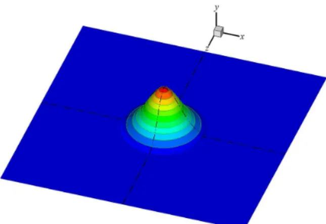
In numerical simulations of the welding processes, the heat input of the arc is modeled by a traveling of a heat source. In this study, this heat source is a two-dimensional Gaussian distribution (Figure 1). Therefore, the heat
flux distribution on the surface of the solid is related to the radial position r= x2+z2(whose reference origin is the arc center that moves with the torch). The Gaussian heat flux distribution considering the torch perpendicular to the plates is given by Equation 5 (Pavelic et al., 1969):
2 2
( /2 )
( ) me r
q r =q − σ (5)
where q(r) is the surface lux at radius r, qm=
η
UI 2πσ
2 is the maximum heat lux in the source center, η is theeiciency coeicient, U is the voltage, I is the current and σ is the radial distance from the center. The surface lux
is reduced by 5% when the r = 2.45σ, which is considered the efecive radius of the circular surface heat source,
Figure 1. Sketch of Gaussian heat input source distribution.
derived from the maximum surface width of the molten zone (Goldak, and Akhlaghi, 2005). Thus, in this study, the heat applicaion concentrates in a circular zone with a radius equal to RAC = 2.45σ.
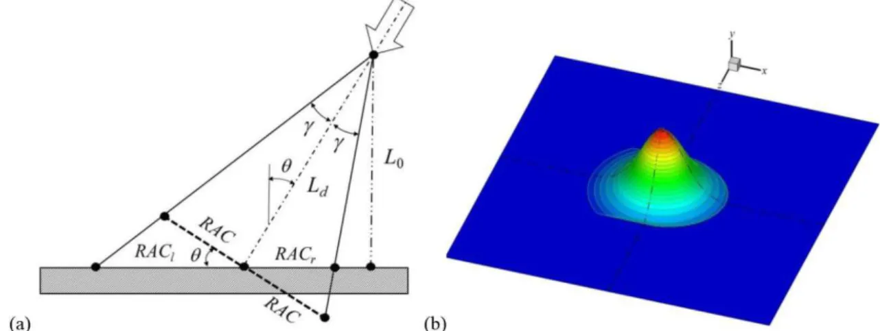
2.2. Proposed heat input source models applied to welding with magnetic arc deflection
shown in Figure 2a. In the second proposal (PM2), instead of using this projection, the radius of heat application (RAC) is modified, as shown in Figure 2b.
In PM1, the heat input is distributed on a virtual plane (Figure 2a), that is perpendicular to the inclined arc, and only the perpendicular component of the heat flux is considered to be imposed on the plates, as shown in Figure 3. Radius r is modified according to the left or right position on the plate surface in relation to the source center C. Therefore, the heat input distribution is more concentrated on the right side and more spread on the left one, as expected in these cases. For an x transversal position of the point, the ones that must be considered in the heat source equation, xl and xr, which are positions on the left and right sides, respectively, are determined by the following Expressions 6 and 7:
cos
lx = x
θ
(6)1
(cos ) r
x = x
θ
− (7)Therefore, the heat input source distribution of PM1 may be given by Equation 8:
2 2
-r 2 2
UI
q(r)= cos .e 2
σ
η
θ
σ π
(8)A sketch of the heat input source considered in PM1 is shown in Figure 3b. The asymmetry of the distribution on the plane, in which the magnetic deflection is imposed, should be noticed.
Figure 2. Sketches of proposed heat source models: (a) PM1 and (b) PM2.
Figure 4 shows sketches of the heat flux and its distribution on the plates considered by PM2. Hongyuan et al. (2005) and Chen et al. (2014) proposed a similar method in which each arc ray, from the electrode tip to the plate surface, rotates according to the arc inclination. Therefore, RAC is modified differently on the left and right sides of the arc center, but keeping the Gaussian angle γ equal to the non-deflected arc one, that is shown in Equation 9.
tan = r RAC
L
γ
(9)where Lr = L0/cosθ is the delected arc length and L0 is the distance from the electrode ip to the plate surface.
Figure 4. Sketches of the heat flux (a) and its distribution (b) on the plates considered by PM2.
Considering RACl and RACr values of RAC on the left and right sides of the arc center, respectively, they can be determined by means of the trigonometric ratios of right triangles, as shown in Equations 10 and 11.
[ tan ( + )sin + cos ]
lRAC = RAC
γ θ
θ
θ
(10)R =
tan sin +cos r
RAC AC
γ θ
θ
(11)Therefore, the heat application zone in PM2 is an ellipse, rather than a circle in conventional Gaussian heat source. Points inside this zone are subject to the heat input and must satisfy the following condition:
2 2
2 2 1
i
x z
RAC + RAC ≤
(12)
where x and z are coordinates of the point under analysis, i is l (let) and r (right). Thus, in this method, (5) is used on both sides (let and right), but taking into account the constraint of ellipse boundaries described in Equaion 12.
2.3. Case studies
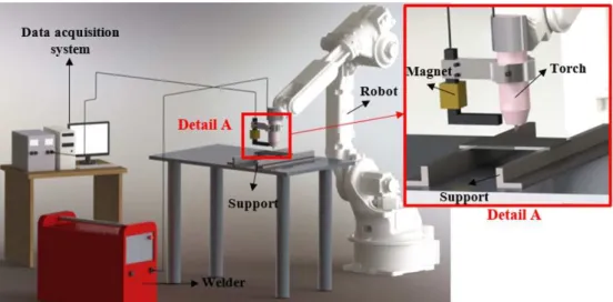
The distance from the electrode tip to the plate surface is 6 mm and the argon shielding gas with flow rate of 13 l/min is used. The mean current and voltage are 100 A and 15 V, respectively. Two experiments are carried out: without arc deflection and with magnetic arc deflection which is kept straight during welding (see Figure 6b and Figure 6c). Temperatures at three points are measured by thermocouples (type K) located at the opposite face of the weld at the middle of the plates in longitudinal direction; one is located at the center line and the others are 5 mm from the center line. They are attached to the metal plate with the use of a capacitive discharge. The data acquisition measurement system is the NI9211 model of National Instruments (accuracy < 0.07K) with 3.5 sample/s/channel and resolution of 24 bits. The transversal section of the fusion zone is obtained by cutting the welded plate which receives a chemical attack with nital 3% to the macrography analysis.
A solenoid is connected to the torch to induce a magnetic field in the arc and to cause its transversal deflection (Figure 6a). The deflection direction (right or left sides) and the arc inclination depend on the voltage applied to the solenoid. In this case, the voltage is 4 V that causes an arc inclination of 25º, which is measured by means of the arc center line drawn on images captured by a high-speed camera (Kang and Na, 2002).
After the comparison of results of both models and the experimental ones found in the first case study, a second case is analyzed to validate the proposed models for welding with weaving by magnetic deflection of the arc, whose experiments were conducted by Larquer and Reis (2016). This case study consists in an autogean bead-on-plate GTAW process, which is applied to SAE 1020 steel plates that are 3 mm thick, 200 mm long and 60 mm wide. The welding speed is 20 cm/min, the distance from the electrode tip to the plate surface is 6 mm and the mean current and voltage are 200 A and 14 V, respectively, for both cases (with and without weaving). The inclination angle is 37.4°. The weaving cycle, whose frequency is 1 Hz, has intervals of 250 ms at the center, Figure 5. Sketch of the system used in the experiments in case 1.
300 ms on the left, 200 ms on the right and 250 ms at the center. Results of width and superficial appearance of the weld bead obtained by Larquer and Reis (2016) are compared to the ones obtained by numerical simulation in both proposed models.
2.4. Mathematical model
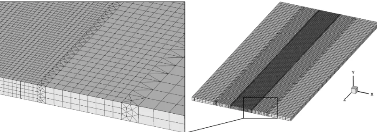
Numerical simulations are carried out by using ANSYS Multiphysics, which solves the transient thermal equations, described in Section 2.1, based on the FEM. Geometries of computational domains are identical to those used in experiments. Room temperature is 30 °C, which is imposed as initial condition for plate materials. Heat transfers for convection and radiation are imposed on all external plate surfaces. Hexahedral elements with eight nodes and surface elements to impose the convection and radiation conditions are employed. Meshes have 171043 nodes and 164576 elements, in the first case study, and 130909 nodes and 121516 elements, in the second one. Figure 7 shows the mesh used in case 1. The element size in the central region, from the welding line up to 15 mm, in both sides, is 0.5 mm, whereas it is 2 mm away from this zone. The mesh used in case 2 has the same shape and element size as the one in case 1. The central region in case 2 comprises the zone from the welding line up to 8 mm in both sides.
Figure 7. Mesh of the computational domain in case 1.
The radial distance from the center (σ) used in the Gaussian heat source model and the efficiency (η) are set for each case, in the validation process, to reach the best temperature curve adjustment and the fusion zone in relation to the experimental ones. Thermal properties of the steel SAE 1020 used in numerical simulations of both cases are temperature dependent. Figure 8 shows the relation between enthalpy (H), thermal conductivity (k), specific mass (ρ) and temperature (Miettinen, 1997). Emissivity is εr = 0.8 whereas the coefficient of convective heat transfer is hc = 8 W/m2 °C (Smith and Smith, 2009).
3. Results and Discussion 3.1. Case 1
In this Section, numerical results considering deflected and non-deflected arcs are compared with experimental ones. Images of the electric arc in both cases are shown in Figure 9. The distorted shape of the deflected arc shows the influence of the magnetic field on the behavior of the arc and, consequently, on the heat input imposed on the plate.
for setting the arc efficiency (η) and the radial distance from the center (σ), which are both degrees of freedom of the Gaussian heat source model. In general, researchers adopt a mean value of the arc efficiency in the numerical simulation without the necessity of any calibration. However, arc efficiency depends on process variables, such as welding velocity, arc length, current, voltage and base material (Niles and Jackson, 1975; Zain-Ul-Abdein, 2009; Arevalo and Vilarinho, 2012). This dependence provides a wide range of arc efficiency values that can be used in numerical simulations by means of heat source models. Grong (1997), for example, reports values of arc efficiency from 25 to 75% for the GTAW process in steel by using argon shielding gas. Therefore, the method of calibration adopted by this study is robust because arc efficiency is also calibrated together with the radial distance from the center. Besides, it is accurate, since it uses both thermocouple temperatures and weld pool boundary obtained experimentally.
After few attempts, η = 49% and σ =1.8 mm and 1.9 mm for 3.2 mm and 6 mm thick plates, respectively, are found. This efficiency agrees with the range studied by Niles and Jackson (1975) and Zain-Ul-Abdein (2009). Temperature distribution on the plate 3.2 mm thick at four instants along the welding process for non-deflected arc is shown in Figure 10. As expected, high temperatures are concentrated around the heat source as it moves. Also, rear zones have higher temperatures in relation to others along the welding.
Figure 8. Thermal properties of steel SAE 1020.
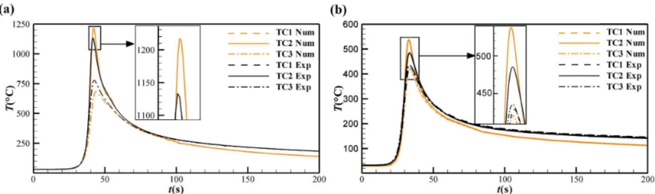
Figure 11 shows thermal cycles for non-deflected case on thermocouple positions (Figure 6b) for 3.2 mm and 6 mm thick plates (Figure 11a and 11b, respectively). The maximum temperature in TC2 is higher than in TC1 and TC3, as expected. It occurred in experimental results of both plates (3.2 mm and 6 mm thick). Temperatures are higher on the 3.2 mm thick plate, since temperatures are measured on the backside of the plates. The numerical model captures the cooling process adequately, since the curve inclinations, after the temperature peak, are close to experimental ones. Table 1 shows maximum temperatures obtained by the model and their differences from experimental ones (ΔTne). Differences vary from 1.8% to 11.9%. Taking into account uncertainties of experiments and the numerical model, including thermal properties, these differences are acceptable.
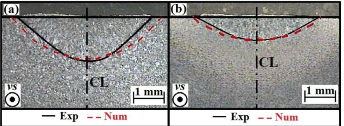
Figure 12 shows the fusion zones obtained for both plate thicknesses, (a) 3.2 mm and (b) 6 mm. Values of width and penetration depth and their differences from experimental ones (ΔLne and ΔPne, respectively) are shown in Table 2. It should be pointed out that numerical results are very close to the ones obtained experimentally, Figure 10. Temperature distribution at four instants along the welding for non-deflected arc: (a) 2.8 s, (b) 12.0 s, (c) 32.0 s and (d) 60.0 s on 3.2 mm thick plate in case 1.
Figure 11. Thermal cycles at TC1, TC2 and TC3 in the non-deflected case on (a) 3.2 mm and (b) 6 mm thick plates in case 1.
Table 1. Maximum temperatures at TC1, TC2 and TC3 in the non-deflected arc in case 1.
Thickness (mm) TC1 (°C) ΔTne (%) TC2 (°C) ΔTne (%) TC3 (°C) ΔTne (%)
3.2 685 11.9 1218 7.5 685 11.9
especially for 6 mm thick plate. In the case of 3.2 mm thick plate, the highest distance between numerical and experimental fusion zone boundaries is found on the plate surface (around 0.40 mm) and, for 6 mm thick plate, it is 0.19 mm, located at half depth.
Temperature distribution on 3.2 mm thick plate at four instants along the welding process of the deflected arc is shown in Figure 13. The behavior of the temperature distribution is similar to the non-deflected one, except the smooth asymmetry observed when the arc is deflected.
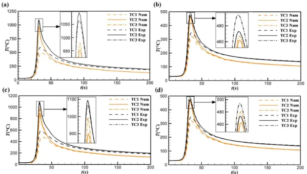
Figure 14 shows thermal cycles obtained in deflected cases: (a) and (b) when PM1 is applied to 3.2 mm and 6 mm thick plates, respectively, and (c) and (d) when PM2 is applied to 3.2 mm and 6 mm thick plates, respectively. An asymmetry on the temperature distribution is captured by thermal cycles at TC1 and TC3, located at the same distance from the centerline of the plate; however, one is on the left and the other on the right side, in both proposed models. In this case, the maximum temperature at TC3 is higher than at TC1 and similar to the one at TC2,
Figure 12. Weld pools obtained experimentally and numerically in the non-deflected case on (a) 3.2 mm and
(b) 6 mm thick plates in case 1 (CL = center line).
Figure 13. Temperature distribution at four instants along the welding in the deflected arc case: (a) 2.8 s, (b) 12 s, (c) 32 s and (d) 60 s on 3.2 mm thick plate in case 1.
Table 2. Width and penetrated depth for fusion zones in the non-deflected arc in case 1.
Thickness (mm) Width (mm) ΔLne (mm) Penetrated depth (mm) ΔPne (mm)
3.2 5.22 0.70 1.44 0.14
located at the centerline of the plate, as occurs in experimental results. Temperature curves obtained numerically and experimentally are very similar at the three positions. These results show the applicability of both proposed models to the magnetic arc deflection.
Table 3 shows maximum temperatures obtained numerically at each point and the difference between numerical and experimental results (ΔTne). A good agreement is found between both proposed models and experiments. In general, both proposed models show better results in 6 mm thick plate, whose differences are from 2.1% to 8.3%, while, in 3.2 mm thick plate, they are from 6.8% to 16.1%. This is because, in the thinner plate, the thermal gradients are high, even in the bottom of the plate, that can lead to errors in the thermocouples results with little position deviation (Smith and Smith, 2009). In 3.2 mm thick plate, PM1 has values smoothly closer at TC1 and TC2, while, at TC3, PM2 reaches better results. In 6 mm thick plate, both models are similar at TC1 and TC2 and PM2 has closer values at TC3.
Figure 14. Thermal cycles at TC1, TC2 and TC3 in the non-deflected case. (a) and (b) for PM1, and (c) and (d) for PM2 applied to 3.2 mm and 6 mm thick plates, respectively.
Table 3. Maximum temperatures at TC1, TC2 and TC3 of PM1 and PM2 in case 1.
Thickness (mm) Model TC1 (°C) ΔTne (%) TC2 (°C) ΔTne (%) TC3 (°C) ΔTne (%)
3.2 PM1 488 14.7 935 6.8 961 9.1
PM2 479 16.1 900 10.3 993 6.1
6 PM1 321 8.3 462 2.4 467 5.5
PM2 320 8.3 463 2.1 480 2.7
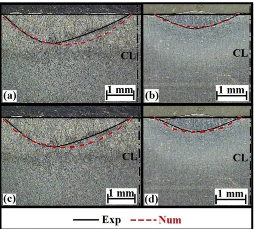
Figure 15 shows weld pool zones numerically and experimentally obtained in the deflected arcs applied to 3.2 mm and 6 mm thick plates: (a) and (b) for PM1 and (c) and (d) for PM2, respectively. In general, numerical results reproduce adequately the shapes of the fusion zones; only the numerical boundary is slightly more rounded than the experimental one. Penetrated depths and bead widths obtained numerically are very close to the experimental ones for both cases. The asymmetry of the weld pool zone in the deflected arc is captured by both models, even this effect been more evident for the thinner plate.
numerical and experimental fusion zone boundaries is found in plate 3.2 mm thick, that reach around 0.17 mm and 0.23 mm (for PM1 and PM2, respectively) in the intermediate depth for both models. These distances are lower for plate 6 mm thick, where the highest distances are around 0.14 mm and 0.12 mm (for PM1 and PM2, respectively) in the intermediate depth. These results show the applicability of both proposed heat source models on the welding with magnetic arc deflection.
3.2. Case 2
In the second case study, fusion zones are analyzed by means of the width and visual presentation of the bead surface, whose experimental results are shown in Larquer and Reis (2016) and Larquer et al. (2016). Firstly, experimental results of the same case, but without weaving, are used to set the parameters σ and η. Figure 16 shows a comparison between the weld beads numerically and experimentally obtained in the non-deflect arc case. The weld bead obtained numerically presents an expected symmetry and it is in good agreement with experiments. After some attempts, σ and η are set 3 mm and 45%, respectively.
A comparison of weld beads numerically and experimentally obtained by welding with weaving by using PM1 and PM2 are shown in Figure 17. The wavy shape of the weld bead edge is well reproduced by both proposed models. Figure 15. Weld pools experimentally and numerically obtained in the deflected arcs applied to 3.2 mm and 6 mm thick plates: (a) and (b) in PM1 and (c) and (d) in PM2, respectively (CL = center line).
Table 4. Width and penetrated depth in the fusion zones in case 1.
Thickness (mm) Model Width (mm) ΔLne (mm) Penetrated depth (mm) ΔPne (mm)
3.2 PM1 4.72 0.16 1.11 0.06
PM2 4.69 0.13 1.08 0.03
6 PM1 3.52 0.25 0.56 0.08
However, there are small spaces between two peaks on the right side of the weld bead obtained numerically that is not seen in experimental ones. This difference may be due to the fact that the force exerted by the arc pressure drags the molten pool which is not possible to be predicted by this type of numerical models. Little differences in the wave shapes are found between models, but both presents these small spaces.
Figure 16. Weld bead numerically (red dashed line) and experimentally obtained in the non-deflect arc in case 2.
Figure 17. Weld bead numerically obtained, (a) PM1 and (b) PM2, and comparison with experimental results in
the deflect arc in case 2.
Table 5. Weld bead widths in the welding with weaving in case 2.
Experimental PM1 Difference (%) PM2 Difference (%)
Lr (mm) 4.71 4.67 0.7 4.77 1.3
Ll (mm) 5.00 5.80 16.0 5.88 17.6
L (mm) 9.71 10.47 7.8 10.65 9.7
of the arc deflection and at the welding center line were very similar. Weld pools were adequately reproduced by the simulations. The widths and penetrated depths obtained numerically were close to the experimental ones for both cases and by both proposed models.
Secondly, numerical results of welding with weaving were compared to experimental ones showed in Larquer and Reis (2016) and Larquer et al. (2016), for both proposed models. Results obtained by numerical simulations were close to the experimental ones and represented adequately the wavy edges of weld beads that are characteristics of these types of welding.
This study shows the capacity of the proposed heat source models to deal with welding subjected to the weaving by means of magnetic arc deflection. The only two degrees of freedom, inherent of the formulation of proposed modified Gaussian heat source models, is a great advantage in the calibration process. Besides, they showed good accuracy when applied to welding with weaving.
Acknowledgements
The first author acknowledges the support of CAPES for the post-graduate scholarship. The authors thank laboratory of research in welding engineering (LAPES – FURG), where this research project was conducted, and Ruham Pablo Reis, Doctor, a professor of Faculdade de Engenharia Mecânica at Universidade Federal de Uberlândia, for providing experiments of welding with weaving.
References
Arevalo HDH, Vilarinho LO. Desenvolvimento e avaliação de calorímetros por nitrogênio líquido e fluxo contínuo para medição de aporte térmico. Soldagem e Inspeção. 2012;17(3):236-250. http:// dx.doi.org/10.1590/S0104-92242012000300008.
Chen Y, He Y, Chen H, Zhang H, Chen S. Effect of weave frequency and amplitude on temperature field in weaving welding process. International Journal of Advanced Manufacturing Technology. 2014;75(5-8):803-813. http://dx.doi.org/10.1007/ s00170-014-6157-0.
Farias RM, Teixeira PRF, Araújo DB. Thermo-mechanical analysis of the MIG/MAG multi-pass welding process on AISI 304L stainless steel plates. Journal of the Brazilian Society of Mechanical Sciences and Engineering. 2017;39(4):1245-1258. http://dx.doi. org/10.1007/s40430-016-0574-y.
Goldak JA, Akhlaghi M. Computational welding mechanics. New York: Springer Science & Business Media; 2005.
Goldak J, Chakravarti A, Bibby M. A new finite element model for welding heat sources. Metallurgical Transactions. B, Process Metallurgy. 1984;15(2):299-305. http://dx.doi.org/10.1007/ BF02667333.
Grong O. Metallurgical modelling of welding. London: Institute of Materials; 1997.
Hongyuan F, Qingguo M, Wenli X, Shude J. New general double ellipsoid heat source model. Science and Technology of Welding and Joining. 2005;10(3):361-368. http://dx.doi. org/10.1179/174329305X40705.
Hu H, Argyropoulos SA. Mathematical modelling of solidification and melting: a review. Modelling and Simulation in Materials Science and Engineering. 1996;4(4):371-396. http://dx.doi. org/10.1088/0965-0393/4/4/004.
Hu JF, Yang JG, Fang HY, Li GM, Zhang Y. Numerical simulation on temperature and stress fields of welding with weaving. Science and Technology of Welding & Joining. 2006;11(3):358-365. http://dx.doi.org/10.1179/174329306X124189.
Hussain B, Sherif El-Gizawy A. Development of 3D Finite Element Model for Predicting Process-Induced Defects in Additive Manufacturing by Selective Laser Melting (SLM). In: International Mechanical Engineering Congress and Exposition; 2016; Phoenix, Arizona. New York: ASME; 2016. (vol. 2: Advanced Manufacturing).
Kang YH, Na SJ. A study on the modeling of magnetic arc deflection and dynamic analysis of arc sensor. Welding Journal. 2002;81(1):8S-13S.
Kang YH, Na SJ. Characteristics of welding and arc signal in narrow groove gas metal arc welding using electromagnetic arc oscillation. Welding Journal. 2003;82(5):93S-99S.
Khurram A, Hong L, Li L, Shehzad K. Prediction of Welding Deformation and Residual Stresses in Fillet Welds Using Indirect Couple Field FE Method. Research Journal of Applied Sciences. Engineering and Technology. 2013;5(10):2934-2940.
2008;29(10):1904-1913. http://dx.doi.org/10.1016/j. matdes.2008.04.044.
Larquer TR, Reis RP. Gas tungsten arc welding with synchronized magnetic oscillation. In: Mahadzir I, editor. Joining technologies. Croatia: InTech; 2016. p. 53-76. (vol. 1).
Larquer TR, Souza DM, Reis RP. Soldagem TIG com oscilação magnética sincronizada. Soldagem & Inspeção. 2016;21(3):363-378. http:// dx.doi.org/10.1590/0104-9224/SI2103.11.
Lim YC, Yu X, Cho JH, Sosa J, Farson DF, Babu SS, et al. Effect of magnetic stirring on grain structure refinement Part 2–Nickel alloy weld overlays. Science and Technology of Welding & Joining. 2013;15(5):400-406. http://dx.doi.org/10.1179/1362 17110X12720264008231.
Miettinen J. Calculation of solidification-related thermophysical properties for steels. Metallurgical and Materials Transactions. B, Process Metallurgy and Materials Processing Science. 1997;28(2):281-297. http://dx.doi.org/10.1007/s11663-997-0095-2.
Niles RW, Jackson CE. Weld thermal efficiency of the GTAW process. Welding Journal. 1975;54(1):25.
Pavelic V, Tanbakuchi R, Uyehara OA, Myers PS. Experimental and computed temperature histories in gas tungsten arc welding of thin plates. Welding Journal Research. 1969;48(Suppl):295s-305s.
Smith MC, Smith AC. NeT bead-on-plate round robin: comparison of transient thermal predictions and measurements. International Journal of Pressure Vessels and Piping. 2009;86(1):96-109. http://dx.doi.org/10.1016/j.ijpvp.2008.11.016.
Sundaresan S, Ram GJ. Use of magnetic arc oscillation for grain
refinement of gas tungsten arc welds in α–β titanium alloys.
Science and Technology of Welding and Joining. 1999;4(3):151-160. http://dx.doi.org/10.1179/136217199101537699.
Teixeira PRF, Araújo DB, Cunha LAB. Study of the Gaussian distribution heat source model applied to numerical thermal simulations of TIG welding processes. Science & Engineering Journal. 2014;23(1):112-115.
Venkatkumar D, Ravindran D. 3D finite element simulation of temperature distribution, residual stress and distortion on 304 stainless steel plates using GTA welding. Journal of Mechanical Science and Technology. 2016;30(1):67-76. http://dx.doi.org/10.1007/ s12206-015-1208-5.