Braz. J. Chem. Eng. vol.31 número2

(1)

ISSN 0104-6632 Printed in Brazil

www.abeq.org.br/bjche

Vol. 31, No. 02, pp. 483 - 495, April - June, 2014 dx.doi.org/10.1590/0104-6632.20140312s00002287

Brazilian Journal

of Chemical

Engineering

LOCAL LINEAR MODEL TREE AND

NEURO-FUZZY SYSTEM FOR MODELLING AND

CONTROL OF AN EXPERIMENTAL pH

NEUTRALIZATION PROCESS

G. Petchinathan

1*

, K. Valarmathi

2

, D. Devaraj

1

and T. K. Radhakrishnan

3

1_{Department of Instrumentation and Control Engineering, Kalasalingam Academy}

of Research and Education, Krishnankoil, Tamilnadu, India. Pin Code - 626 126, Phone: + 91 90035 23312, Fax: + 91 4563 289322.

E-mail: gpetchi@gmail.com

2

P. S. R. Engineering College, Sivakasi, Tamilnadu, India. E-mail: krvalarmathi@yahoo.co.in

3

Department of chemical Engineering, National Institute of Technology, Trichy, Tamilnadu India.

E-mail: radha@nitt.edu

(Submitted: September 19, 2012 ; Revised: April 4, 2013 ; Accepted: July 23, 2013)

Abstract - This paper describes the modelling and control of a pH neutralization process using a Local Linear Model Tree (LOLIMOT) and an adaptive neuro–fuzzy inference system (ANFIS). The Direct and Inverse model building using LOLIMOT and ANFIS structures is described and compared. The direct and inverse models of the pH system are identified based on experimental data for the LOLIMOT and ANFIS structures. The identified models are implemented in the experimental pH system with IMC structure using a GUI developed in the MATLAB -SIMULINK platform. The main aim is to illustrate the online modelling and control of the experimental setup. The results of real-time control of an experimental pH process using the Internal Model Control (IMC) strategy are also presented.

Keywords: LOLIMOT; ANFIS; Internal Model Control; pH process.

INTRODUCTION

Control of pH plays a very important role in chemical industries, such as wastewater treatment, polymerization reactions, fatty acid production, bio-chemical processes, etc. Modelling and control of a pH process is a very challenging and extremely com-plex task, because the slope of the process nonlinear-ity can be very steep around the neutralization region and small changes in the influent stream concentra-tion can result in tremendous changes in pH (Rodrigues and Loparo, 2004). It is very difficult to achieve high performance and robust control using

(2)

Brazilian Journal of Chemical Engineering

(Nahas et al., 1992) and model predictive control (Richalet, 1993) schemes can be employed to im-prove the closed loop performance of the system. Due to the complexity of the industrial process, a first- principles model cannot be applied and hence a more flexible type of model needs to be used. In recent decades, numerous schemes have been used for modelling and control of nonlinear processes. The genetic algorithm (GA) approach is used to find the optimal values of the model parameters and controller parameters for modelling and control of complex nonlinear process (Mwembeshi and Kent, 2004 ; Valarmathi et al., 2009). The response time is high in the case of the GA based approach. The multi-layer artificial neural network (ANN) was introduced in the 1980s. It allows fast processing of large amounts of information. A large repository of literature using ANNs and their application in many different fields like modelling and control are avail-able. The ANNs are also used in system identifica-tion and control of pH processes (Sean, 1999; Wior et al., 2010; Sivaraman and Arulselvi, 2011). Radhakrishnan et al. (2009) proposed a GA and ANN approach for system identification and control of a pH process. The main problem with the neural based approach is that no human expertise can be stored. The fuzzy logic-based modelling (Babuska and Verbruggen 2003) approach has been widely used in many industrial processes. The main diffi-culty related to fuzzy-based approach is that it needs prior knowledge about the operation of the process.

To overcome the problems associated with individually using fuzzy and neural approaches, a large variety of Neuro-Fuzzy system (NFS) ap-proaches was introduced in the 1990s. Jang (1993) introduced the adaptive neuro–fuzzy inference system (ANFIS), which belongs to a class of NFS. ANFIS is an adaptive network which permits the usage of neural network topology together with fuzzy logic. It not only includes the characteristics of both methods, but also eliminates some disadvan-tages when used alone. Any linear or nonlinear function can be approximated using ANFIS. The NFS has the capacity to store human expertise and learning. In the last decade, NFS has been proposed for modelling and control of complex nonlinear industrial processes (Vieira et al., 2004; Rezaeeian et al., 2008; Wu et al., 2008; Navghare et al., 2011). The fast neural network LOLIMOT was introduced to determine the structure of a local linear input-output model description from experimental data by Nelles (1999). The learning phase of this network is quite fast and more deterministic than a classical

neural network. The response time of a LOLIMOT network is much less. It was proposed for modelling of a heat exchanger (Fischer et al., 1998) and the combustion process of a diesel engine (Hafner et al., 2000) and Van der Vusse reactor (Widjiantoro at al., 2003).

In this study, LOLIMOT and NFS are used to ascertain its effectiveness for modelling and control of an experimental pH neutralization process using MATLAB. The direct and inverse models are ob-tained using both the techniques. The internal model control scheme is used for control of the process.

EXPERIMENTAL SYSTEM: pH NEUTRALIZATION PROCESS

(3)

Local Linear Model Tree and Neuro-Fuzzy System for Modelling and Control of an Experimental pH Neutralization Process 485

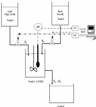
Figure 1: Schematic diagram of the pH neutralization process.

Figure 2: Experimental pH neutralization process.

Figure 3: DAQ Module.

The 0.2 g mol L-1 acid stream of acetic acid (CH3COOH) is pumped into the mixing tank at a

constant flow rate (Fa) with 30% opening of the

con-trol valve. The 0.1 g mol L-1 base stream of sodium hydroxide (NaOH) is pumped into the mixing tank by a pneumatic control valve at a flow rate of Fb.

The stirrer inside the mixing tank is used for mixing of the two streams. A neutral product and salt are produced by reaction between acid and base. The acid flow rate, Fa, introduces the disturbance in the

process and the base stream flow rate, Fb, is used as a

manipulated variable for control of the pH in the mixing tank. In this study, the maximum flow of acid and base streams is maintained around 1.2 L/min. The percentage of opening of the control valve is calibrated as flow rate for acid and base streams.

MODELLING OF THE pH NEUTRALIZATION PROCESS

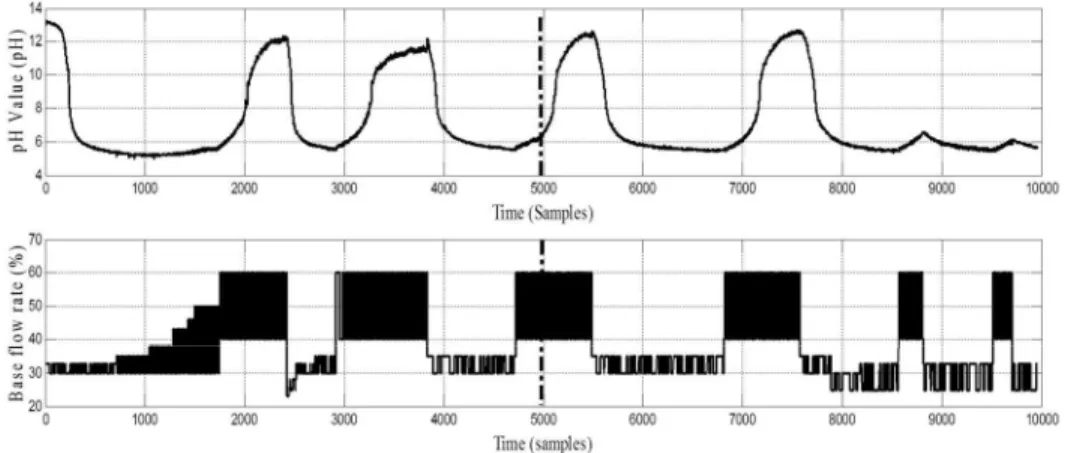
Theoretical modelling of a pH process is too complex because of the severe nonlinear behaviour of the system. As to the characteristics of the experimental pH process, the nominal operating range of pH is from 5 to 12 and the nominal operating range of the base flow rate (Fb) is from

20% to 100% because the minimum value of the base flow rate is only obtained at 20% of the opening of the control valve. Here, the base and acid flow rate are measured in terms of % of the respective control valve opening. For modelling of the pH neutralization process, the acid is pumped into the mixing tank at a constant flow rate (Fa) of 30%

opening of the control valve and the control signal (base flow rate Fb) is varied in the range of 20% to

70% opening of the control valve by a variable amplitude pseudo-random function. For more than 70% opening of the base flow control valve, the pH value of the solution in the mixing tank reaches around 13 and does not reduce further upon variation of the base flow rate for a long period of time. Hence, the operating range of base flow rate Fb was

fixed in the range of 20% to 70% opening of control valve. The training and validation data sets for this study were obtained in an open loop using perturba-tions on the base flow-rate (Fb) as shown in Figure 8,

from which variation of the pH was obtained from 5 to 12.This region exhibits the nonlinear behaviour of the process.

(4)

of the system is constant and equal to one sampling period. The structures of the direct and inverse models for training are illustrated in Figures 4 and 5. These structures are the main solutions for training models illustrated in the literature (Deshpande and Ash, 1988; Hunt and Sbarbaro, 1991). The represen-tation of a nonlinear dynamic system using the black–box approach at discrete time k + 1 is a non-linear function of past inputs (nu) and past outputs

(ny) and noise and is in the form of a NARX

(Nonlinear Auto Regressive with Exogenous inputs) model, given by Eq. (1)

( 1), ( 2)... ( ),

( ) ( )

( 1), ( 2),... ( )

y

u

y k y k y k n

y k f e k

u k u k u k n

− − −

⎛ ⎞

= _⎜ ₋ ₋ ₋ _⎟+

⎝ ⎠ (1)

In the above equation, ny and nu represent the

number of previous output samples used and the number of previous control (input) signal samples used, respectively. The direct and inverse models of the pH process are obtained with ny= nu= 2. The

values of ny, nu and time delay (nk) are evaluated

using the system identification toolbox of MATLAB based on statistical criteria, viz., the Akaike informa-tion criterion (AIC) and Final Predicinforma-tion Error (FPE) value, as shown in Table 1.

Figure 4: Structure of the direct model for training.

Figure 5: Structure of the inverse model for training. The prediction of the pH in the direct model of the process at time k is given by Eq. (2).

( ) ( ( 1), ( 2),

( 1), ( 2))

ypred k f y k y k

u k u k

= − −

− − (2)

The prediction of the control signal at time instant

k in the inverse model is given by Eq. (3)

( ) ( ( ), ( 1), ( ),

( 1), ( 2))

upred k g y k y k r k

u k u k

= −

− − (3)

where r(k) is the reference signal at time k. The local linear model tree (LOLIMOT) and neuro-fuzzy systems approaches like ANFIS were used to obtain the direct and inverse models of the nonlinear pH process.

Table 1: FPE and AIC for different values of ny,

nu and nk.

Model nu ny nk FPE AIC

M1 1 1 1 0.0023 -6.0731

M2 2 2 1 0.0017 -6.3762

M3 3 2 1 0.0017 -6.3520

M4 3 3 1 0.0017 -6.3485

M5 4 3 1 0.0018 -6.3421

M6 4 4 1 0.0017 -6.3704

M7 5 2 1 0.0018 -6.3096

M8 5 5 1 0.0017 -6.3096

Local Linear Model Tree

Local Linear Model Tree (LOLIMOT) is one kind of fast local linear neural networks, because the learning phase is quite fast and more deterministic than a classical neural network. This network was introduced by Nelles (1999). The main idea of this network is to approximate the non-linear function with multiple piecewise linear models. It is an extended radial basis function network and it is obtained by replacing the output layer weights with a linear function of the network inputs. Thus, each neuron represents a local linear model with its corresponding validity function. In addition to this, the radial basis function network is normalized, that is, the sum of all validity functions for a specific input combination sums up to one. The local linear models are interpolated by Gaussian functions as the weighing functions. The Gaussian weighing func-tions determine the regions of the input space where each neuron is active. The input space of the net is divided into M hyper-rectangles, each represented by a linear function (Hafner et al. 2000).

The output y of the LOLIMOT network with p inputs u₁,u₂...u_pis calculated by summing up the contributions of all M local linear models.

0 1 1 2 2

1

ˆ ( ... )

( , , )

M

i i i ip p

i

i i i

y w w u w u w u

u c =

= + + + +

Φ σ

∑

(5)

Local Linear Model Tree and Neuro-Fuzzy System for Modelling and Control of an Experimental pH Neutralization Process 487 where wik are the parameters of the i

th

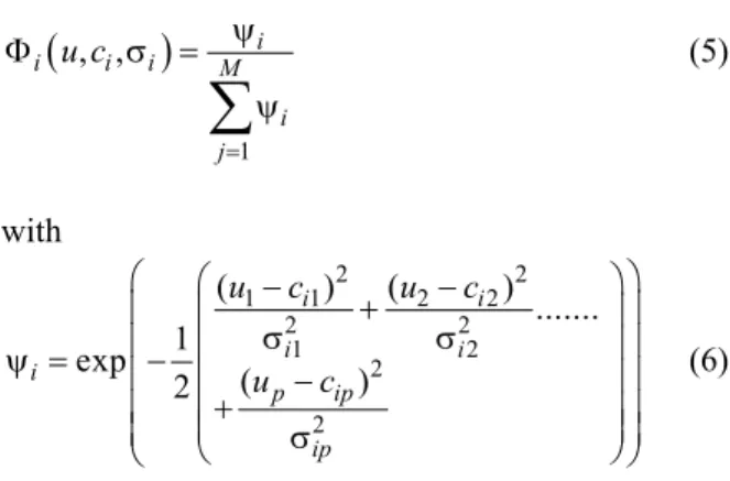
linear regres-sion model, u is the input vector and Φiis the

nor-malized Gaussian weighing function for the ith model with center coordinate ci and standard deviations σi.

(

)

1

, , i

i i i M

i j

u c

=

ψ

Φ σ =

ψ

∑

(5)

with

2 2

1 1 2 2

2 2

1 2

2 2

( ) ( )

... 1

exp

( )

2

i i

i

p ip

ip

u c u c

u c

⎛ ⎛ − ₊ − ⎞⎞

⎜ ⎜ ⎟⎟

σ σ

⎜ ⎜ ⎟⎟

ψ = _⎜− _⎜ ₋ _⎟_⎟

+

⎜ ⎜_⎜ ⎟_⎟⎟

⎜ _⎝ σ _⎠⎟

⎝ ⎠

(6)

The procedure of this network is split into two loops. In the outer loop, the structure of the local model network is optimized for the number of neurons and the partitioning of the input space. The network structure is optimized by a tree construction algorithm that determines the centers and standard deviations of the weighing functions (Figure 6). The inner loop estimates the parameters and structure of the local linear models by a local modelling tech-nique (Pedram et al., 2006).

The LOLIMOT network partitions the input space in hyper rectangles. The weighting function of the corresponding linear model is placed in the

center of each hyper rectangle. The standard devia-tions are selected proportional to the size of the hyper rectangle. This creates the size of the validity region of a local linear model proportional to its hyper rectangle extension. A model may be valid over a wide operating range of one input variable but only in a small range of another one.

At the outer loop of the each iteration, the local linear model with the worst local error in Eq. (7) is bisected into two new ones. Local error is the sum of the squared errors weighted with the corresponding weighing function Φi over all the data samples N.

2 1

ˆ ( ( )) ( ( ) ( ))

N

local i

j

J u j y j y j

=

∑

Φ − (7)

The possible cuts in all dimensions are tested and the one with the highest performance is selected as a new hyper rectangle. In the inner loop, the parame-ters of the local linear models are calculated by a local weighted least-squares technique. Some unique features of the LOLIMOT network are, local estima-tion of the local linear model parameters, considering only the worst local linear model for a split and freezing of the validity function values for extrapola-tion. This network is very fast and robust. In addition, the computational demand increases only linearly with the number of local models due to the local estimation approach (Widjiantoro et al., 2003; Deshpande and Ash, 1988).

(6)

Neuro-Fuzzy System

A fuzzy inference system (FIS) can use human knowledge by storing its crucial components in a rule base, and perform fuzzy reasoning to infer the overall output value. The source of if-then rules and its membership function largely depend on a priori knowledge about the process. On the other hand, there is no logical way to transfer the knowledge of human experts to the knowledge base of a FIS. So, there is a need for adaptation of the rule base to generate the output within the specified error. The combination of FIS and ANN results in the NFS. The NFS takes advantage of the capacity that FIS has to store human expertise and the capacity of learning of the ANN (Vieira et al., 2004). The learning algorithm is applied to a FIS by forming a special ANN-like architecture known as an adaptive neuro-fuzzy inference system (ANFIS). In this paper, ANFIS was taken as the NFS, because of its robustness and fast convergence.

The architecture of the ANFIS (Jang, 1993) is illustrated in Figures 7(a) and 7(b). Assume that the FIS under consideration has two inputs ,u x and one output z. For a first-order Sugeno fuzzy model, a com-mon rule set with two fuzzy if–then rules is as follows in Eq. (8).

Rule 1:

If u is A1 and x is B1, then z₁= p₁u+q₁x+r₁,

Rule 2:

If u is A2 and x is B2, then z₂ = p₂u+q₂x+r₂. (8)

The reasoning mechanism for the Sugeno model is illustrated in Figure 7(a) and the corresponding equivalent ANFIS architecture is shown in Figure 7(b).

The output z in Figure 7(b) can be written as

1 2

1 2 1 2

1 1 1 1 2 2 2 2

1 1 1 1 1 1

2 2 2 2 2 2

( ) ( )

( ) ( ) ( )

w w

z z z

w w w w

w p u q x r w p u q x r

w u p w x q w r

= +

+ +

= + + + + +

= + +

+ + +

(9)

The ANFIS architecture has five layers, as shown in Figure 7(b). The first layer has the membership functions for each input and rule, the second layer determines the firing strength of each rule, and the third layer normalizes the value of the firing strength. The nodes in the fourth layer are adaptive and perform the consequence of the rules. The parameters in this layer are referred to as consequent parameters. Finally, the overall output can be ex-pressed as a linear combination of the resultant parameters in the fifth layer.

(a)

(b)

(7)

Local Linear Model Tree and Neuro-Fuzzy System for Modelling and Control of an Experimental pH Neutralization Process 489 The learning algorithm of ANFIS is composed of

two phases. In the forward phase, the node output values go forward until layer 4 and the resultant pa-rameters are identified by the least squares method. In the backward phase, the output errors are propa-gated backward and the parameters are updated by the gradient descent method.

LOLIMOT and ANFIS Structures for Modelling

The ability of a LOLIMOT network to identify nonlinear systems was ascertained by Nelles (1999) and Widjiantoro et al. (2003). In general, the choice of model structure depends on the projected use of the model. In this study, the model is used for predic-tion purposes. The local linear models are chosen to be the nonlinear ARX (NARX) model. The NARX requires past input signals and past real output sig-nals as an input to form the predicted output. The structure of NARX is very simple and allows the use of linear optimization techniques.

The standard ANFIS structure is used to obtain the direct and inverse model. The structure contains sixteen rules, four inputs with two bell-shaped mem-bership functions and one output that is a linear func-tion of the resultant parameters

The good regressor for LOLIMOT and ANFIS based modelling is obtained via the process of itera-tion with initial values. The regressor is taken as a row vector [nu ny nk]. Here, nu is the number of past

input signals that affects the next output. ny is the

number of past output signals and nk is the time

delay. The initial value of the regressor is taken as [2 2 1] for both techniques, similar to the orders used in the NARX model. The direct and inverse models are obtained with training and test data sets using the LOLIMOT and ANFIS techniques. The identifica-tion procedures use a fuzzy control toolbox for use with MATLAB for the LOLIMOT and ANFIS mod-els (Molsa, 2007).

Comparison of the LOLIMOT and ANFIS Models

The input – output data collected from the ex-perimental pH process are shown in Figure 8. Out of the 10000 samples collected, 5000 samples of data are used for training and the remaining 5000 samples of data are used for validation. The number of ing epochs is fixed. The stopping criterion for train-ing is a minimum value of the mean square error (MSE). In this study, the minimum value of MSE was taken as 1e-6. The MSE was used as the criterion for the training and test data sets to compare the ac-curacy of the model. The simulation results of the direct and inverse model are shown in Tables 2 and 3, respectively. The simulation output of LOLIMOT and ANFIS based direct and inverse models are shown in Figures 9(a)-12(a). The enlarged versions of the simulation output of the LOLIMOT and ANFIS based direct and inverse models are pre-sented in Figures 9(b)-12(b) to illustrate the differ-ence between the mentioned variables.

Figure 8: Training and Validation Data.

Table 2: MSE for the Direct Model.

MSE Direct Model

Training Testing

LOLIMOT 1.620e-3 1.589 e-3

(8)

Table 3: MSE for the Inverse Model.

MSE Inverse Model

Training Testing

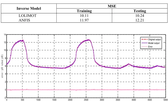
LOLIMOT 10.11 10.24

ANFIS 11.97 12.21

0 500 1000 1500 2000 2500 3000 3500 4000 4500 5000

-2 0 2 4 6 8 10 12 14

Time (samples)

er

ror

/

pH

va

lue

( pH

)

Original output Model output Error

Figure 9(a): LOLIMOT direct model output after validation.

400 420 440 460 480 500

12.2 12.25 12.3 12.35 12.4 12.45 12.5 12.55 12.6

Time (samples)

error /

pH

v

al

u

e(

p

H

)

Figure 9(b): Enlarged View of the LOLIMOT direct model output after validation.

0 500 1000 1500 2000 2500 3000 3500 4000 4500 5000

-2 0 2 4 6 8 10 12 14

Time (samples)

E

rr

o

r / ph

v

a

lu

e(

pH

)

(9)

380 390 400 410 420 430 440 450 460 470

12.15 12.2 12.25 12.3 12.35 12.4 12.45 12.5 12.55 12.6

Time (samples)

E

rro

r /

p

h

v

a

lu

e

(p

H

)

Figure 10(b): Enlarged View of the ANFIS direct model output after validation.

0 500 1000 1500 2000 2500 3000 3500 4000 4500 5000

-20 -10 0 10 20 30 40 50 60 70

Time (Samples)

E

rr

o

r / B

a

s

e

F

lo

w

r

a

te

%

Figure 11(a): LOLIMOT inverse model output after validation.

350 400 450 500 550 600

-20 -10 0 10 20 30 40 50 60

Time (Samples)

E

rr

o

r /

B

a

s

e

F

lo

w

ra

te

%

Figure 11(b): Enlarged view of the LOLIMOT inverse model output after validation.

0 500 1000 1500 2000 2500 3000 3500 4000 4500 5000

-40 -20 0 20 40 60 80

Time (Samples)

E

rr

o

r

/

Ac

id

F

lo

w

r

a

te

( %

)

y p

(a)

(10)

350 400 450 500 550 600

-20 -10 0 10 20 30 40 50 60 70

Time (Samples)

Er

ro

r / Ac

id

F

lo

w

r

a

te

( %

)

(b)

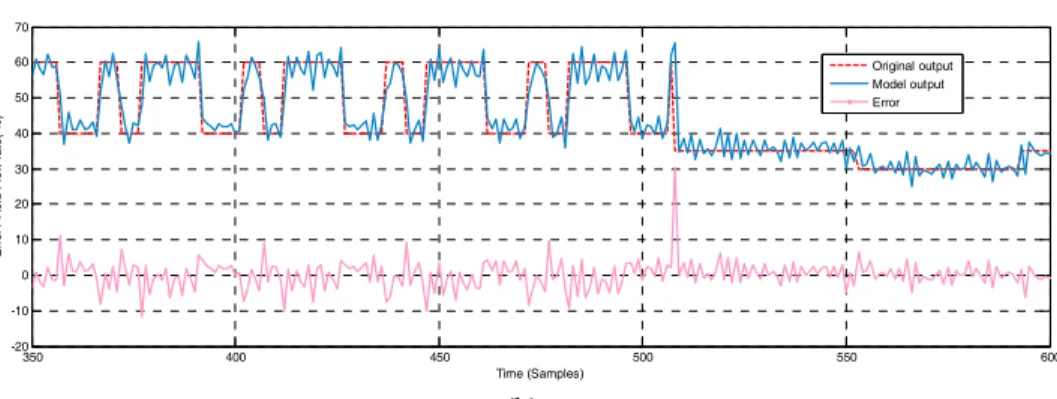
Figure 12(b): Enlarged view of the ANFIS inverse model output after validation.

From Tables 2 and 3, it can be seen that the LOLIMOT structure achieved a smaller MSE com-pared to the ANFIS structure. The obtained models can also be compared in terms of complexity by meas-uring the number of parameters, number of training epochs and training time. The results are summarized in Table 4 for the direct and inverse models. From Table 4, it can be seen that the number of parameters and training time are less in LOLIMOT compared to ANFIS because of the standard ANFIS structure.

Table 4: Complexity comparison.

Direct Model Inverse Model Properties

LOLIMOT ANFIS LOLIMOT ANFIS

No. of

parameters 19 104 37 104

No. of training epochs

100 50 50 50

Training

time (sec) 5 9 8 17

CONTROL OF A pH NEUTRALIZATION PROCESS

To test the obtained direct and inverse models for both the LOLIMOT and ANFIS architectures, the internal model control (IMC) strategy was used. The internal model control (IMC) method was introduced by Garcia and Morari (1985) and thorough research and development took place during the past decades (Garcia and Morari. 1985; Morari and Zafiriou, 1989). The IMC method relies on the internal model principle, which states that if any control system contains within it, implicitly or explicitly, some representation of the process to be controlled, then a perfect control is simply achieved. In particular, if the control scheme has been developed based on the exact model of the process, then perfect control is

theoretically possible. The IMC method includes an internal model and an internal model controller, which consists of the inverse internal model and a filter. It provides good tracking and robust performance.

The standard structure of the IMC scheme, where the process model plays an explicit role in the control structure compared to the standard control loop, is shown in Figure 13. The IMC structure has some advantages over a conventional feedback con-trol loop. For the nominal, the case plant (Gp) is

equal to the plant model (Gpo); for instance, the

feedback is affected only by the disturbance ‘d’, such that the system is effectively under open loop and hence no stability problems can arise. Also, if the process transfer function (Gp) is stable, the closed

loop system is stable for any stable controller, Moreover, the controller can simply be designed as a feed-forward controller in the IMC scheme.

Figure 13: Standard structure of the IMC scheme.

In IMC design, controller GQ can be designed as a

(11)

Figure 14: Structure of the Internal Model Control.

Implementation of IMC in Real-Time Control Action

The controllers are directly tested in the experi-mental pH neutralization process, after the simula-tion results are considered satisfactory. Figures 15

and 16 show the results of LOLIMOT and ANFIS internal model controllers for the experimental pH neutralization process. The real-time control action is performed for four different step changes in set point such as pH values of 7, 8, 9 and 11. The LOLIMOT and ANFIS based IMCs track the reference signal satisfactorily and produce reasonable control inputs.

Minimization of the mean square error (MSE) was used as a metric measure function for comparing the results of these two approaches. In LOLIMOT based IMC, as shown in Figure 15, the control actions for the changes from 7 to 8, 8 to 9 and 9 to 11 are smooth and track the set point with small overshoot, but the pH change from 11 to 9 takes more time to settle down.

Figure 15: IMC using the LOLIMOT based model.

(12)

Overall results of the LOLIMOT based IMC are reasonable. For the ANFIS based IMC, as shown in Figure 16, the control actions for the changes from 7 to 8 and 9 to 11 are reasonably good, but for changes from 8 to 9 and 11 to 9 some oscillations occur in output and also the settling time is high. From Figures 15 and 16, it can be seen that the output is close to the set point, which shows that the model can capture dynamics of the nonlinear process very well. From Table 5, it can be concluded that the LOLIMOT based IMC gave better performance than the ANFIS based IMC.

Table 5: Performance comparison of the controllers.

Controller MSE

IMC - LOLIMOT 0.2235

IMC - ANFIS 0.2475

CONCLUSIONS

In this study, modeling of the experimental pH process is based on LOLIMOT and ANFIS struc-tures and real-time control action is performed using the IMC structure for both the models. In the direct and inverse modelling of the pH process, the MSE of the training and testing are close in the LOLIMOT and ANFIS structures. The error achieved is smaller when using a LOLIMOT than with ANFIS. The time taken for the training is also higher in ANFIS than LOLIMOT because the standard ANFIS structure used is not very flexible. The real time control action using IMC structure with both the approaches pro-duced good results. However, the control action with the LOLIMOT model gives a slightly better result than the ANFIS model. In general, both the ap-proaches are valid options for modelling of complex and non-linear real-time systems.

ACKNOWLEDGEMENT

This work was performed at the Advanced Process Control Laboratory (DST- FIST sponsored), Kalasalingam Academy of Research and Education, Krishnankoil, Srivilliputtur.

REFERENCES

Babuska, R., Verbruggen, H., Neuro-fuzzy methods for nonlinear system identification. Annual Reviews in Control, 27, 73-85 (2003).

Billings, S. A., Identification of nonlinear systems – a survey. Proceedings of IEE, Part D: Control Theory and Applications, 127(6), 272-285 (1980). Deshpande, P. B., Ash, R. H., Computer Process

Control with Advanced Control Applications. 2nd Revised Edition, ISA (1988).

Doherty, S. K., Control of pH in chemical processes using artificial neural networks. Ph.D Thesis, Liverpool John Moores University (1999).

Fink, A., Nelles, O., Isermann, R., Nonlinear internal model control for MISO systems based on local linear neuro-fuzzy models. In Proceedings of 15th Triennial World Congress International Federation of Automatic Control, Barcelona, Spain (2002). Fischer, M., Nelles, O., Isermann, R., Adaptive

predictive control of a heat exchanger based on a fuzzy model. Control Engineering Practice, 6(2), 259-269 (1998).

Garcia, C. E. and Morari, M., Intenal model control-2: Design procedure for multivariable systems. Ind. Eng. Chem. Process Des. Develop., 24(3), pp. 427-484 (1985).

Hafner, M., Schuler, M., Nelles, O., Isermann, R., Fast neural networks for diesel engine control design. Control Engineering Practice, 8, 1211-1221 (2000).

Han, M., Han, B., Guo, W., Process control of pH neutralization based on adaptive algorithm of uni-versal learning network. Journal of Process Control, 16, 1-7 (2006).

Hunt, K. J., Sbarbaro, D., Neural networks for linear internal model control. IEEE Proceedings-D, Control Theory and Applications, 138(5), 431-438 (1991).

Jang, J. S. R., ANFIS: Adaptive-network-based fuzzy inference systems. IEEE Transactions on System, Man, and Cybernetics, 23(3), 665-685 (1993). Molsa, J., Limited toolbox for fuzzy identification

and control for use with MATLAB. Tampere University of Technology (2007).

Morari, M., Zafiriou, E., Robust Process Control. Prentice Hall. Englewood Cliffs, USA (1989). Mwembeshi, M. M., Kent, C. A., Salhi, S., A genetic

algorithm based approach to intelligent modelling and control of pH in reactors. Computers & Chemical Engineering, 28(9), 1743-1757 (2004). Nahas, E. P., Henson, M. A., Seborg, D. E.,

Non-linear internal model control strategy for neural network models. Computers & Chemical Engi-neering, 16, 1039-1057 (1992).

(13)

Local Linear Model Tree and Neuro-Fuzzy System for Modelling and Control of an Experimental pH Neutralization Process 495 Nelles, O., Nonlinear System Identification with

Lo-cal Linear Neuro-Fuzzy Models. Dissertation, Technische Universität Darmstadt, Shaker Verlag, Aachen, (1999).

Pedram, A., Jamali, M. R., Pedram, T., Fakhraie, S. M., Lucas, C., Local linear model tree (LOLIMOT) reconfigurable parallel hardware. International Symposium on Parallel Computing in Electrical Engineering, 13(17), 198-201 (2006).

Radhakrishnan, T. K., Valarmathi, K., Devaraj, D., Intelligent techniques for system identification and controller tuning in pH process. Brazilian Journal of Chemical Engineering, 26(01), pp. 99-111 (2009).

Rezaeeian, A., Yousefi-Koma, A., Shasti, B., Doosthoseini, A., ANFIS modeling and feed for-ward control of shape memory alloy actuators. International Journal of Mathematical Models and Methods in Applied Sciences, 2(2), 228-235 (2008).

Richalet, J., Industrial applications of model based predictive control. Automatica, 29(5), 1251-1274 (1993).

Rodriguez, J. L., Loparo, K. A., Modelling and iden-tification of the pH processes. In Proceedings of the American Control Conference, 6, 5483-5488 (2004).

Sivaraman, E., Arulselvi, S., Neuro modeling and

control strategies for a pH process. International Journal of Engineering Science and Technology, 3(1), 194-203 (2011).

Syafiie, S., Tadeo, F., Martinez, E., Model-free learn-ing control of neutralization processes uslearn-ing rein-forcement learning. Engineering Applications of Artificial Intelligence, 20, 767-782 (2007). Valarmathi, K., Devaraj, D., Radhakrishnan T. K.,

Real-coded genetic algorithm for system identifi-cation and controller tuning. Applied Mathematical Modelling, 33, 3392-3401 (2009).

Vieira, J., Dias, F. M., Mota, A., Artificial neural networks and neuro-fuzzy systems for modelling and controlling real systems: a comparative study. Engineering Applications of Artificial Intelligence, 17, 265-273 (2004).

Widjiantoro, B. L., Liong, T. H., Nazaruddin, Y. Y., Purnama B. S., LOLIMOT Based Model Predictive Control. Jurnal Teknologi, 17(1), 37-44 (2003). Wior, I., Boonto, S., Abbas, H. S., Modeling and

control of an experimental pH neutralization plant using Neural Networks based Approximate Pre-dictive Control. In Proceedings of 1st Virtual Control Conference, Denmark (2010).