http://www.ntmsci.com
On the Mannheim surface offsets
Mehmet ¨Onder1and H. H¨useyin Uˇgurlu2
1Celal Bayar University, Faculty of Arts and Sciences, Department of Mathematics, 45140, Muradiye, Manisa, Turkey.
2Gazi University, Faculty of Education, Department of Secondary Education Science and Mathematics Teaching, Mathematics Teaching Program, Ankara, Turkey.
Received: 27 January 2015, Revised: 4 March 2015, Accepted: 29 May 2015 Published online: 18 June 2015
Abstract: In this paper, we study Mannheim surface offsets in dual space. By the aid of the E. Study Mapping, we consider ruled surfaces as dual unit spherical curves and define the Mannheim offsets of ruled surfaces by means of dual geodesic trihedron (dual Darboux frame). We obtain the relationships between the invariants of Mannheim ruled surfaces. Furthermore, we give the conditions for these surface offsets to be developable.
Keywords: Ruled surface; Mannheim offset; dual angle.
1 Introduction
Generally, an offset surface is offset a specified distance from the original along the parent surface’s normal. Offsetting of curves and surfaces is one of the most important geometric operations in CAD/CAM due to its immediate applications in geometric modeling, NC machining, and robot navigation [4]. Especially, the offsets of ruled surfaces, which are the surfaces generated by continuously moving of a straight line, have an important role in (CAGD) [11,12]. These surfaces are used in different kinds of applications of Computer Aided Geometric Design (CAGD), moving geometry and kinematics. In [13], Ravani and Ku defined and studied the well-known offsets of ruled surfaces called Bertrand trajectory ruled surfaces. Then, K¨uc¸¨uk and G¨ursoy have introduced closed Bertrand trajectory ruled surfaces in dual space in terms of their integral invariants [6]. They have obtained the relations between the pitches and angle of pitches of closed Bertrand trajectory ruled surfaces. Also, they have given some characterizations including the relationships between the area of projections of spherical images and integral invariants of Bertrand trajectory ruled surfaces.
Recently, a new offset of ruled surfaces has been defined by Orbay, Kasap and Aydemir [7]. They have called this new offset as Mannheim offset and studied the developable Mannheim offset surfaces. Later, ¨Onder and Uˇgurlu have defined and studied Mannheim offsets of ruled surfaces in the Minkowski 3-spaceE13[8,9]. Furthermore, Mannheim offsets of closed ruled surfaces in dual space have been studied according to Blaschke frame in [10] and the characterizations of Mannheim offsets of ruled surfaces in terms of integral invariants and areas of projection have been given.
2 Dual representation of ruled surfaces
W.K. Clifford (1845-1879) had been introduced dual numbers such as a dual number is a double in the form ¯
a= (a,a∗) =a+εa∗whereaanda∗are real numbers andε= (0,1)is called dual unit with the property thatε2=0 [1]. Let ¯a= (a,a∗) =a+εa∗and ¯b= (b,b∗) =b+εb∗be two dual numbers. The product of these numbers is defined by
¯
ab¯= (a,a∗)(b,b∗) = (ab,ab∗+a∗b) =ab+ε(ab∗+a∗b). (1)
Then, the set of dual numbers is denoted byD,
D={
¯
a=a+εa∗: a,a∗∈R,ε2=0}
. (2)
Dual differentiable function of a dual variable has been studied by Dimentberg [2]. He derived the following general expression for a dual (differentiable) function
f(x¯) =f(x+εx∗) = f(x) +εx∗f′(x), (3)
wheref′(x)shows the derivative of f(x)with respect tox. From this definition, we can give the following dual expressions for some well-known functions,
cos(x¯) =cos(x+εx∗) =cos(x)−εx∗sin(x), sin(x¯) =sin(x+εx∗) =sin(x) +εx∗cos(x),
√
¯
x=√x+εx∗=√x+ε x∗
2√x, (x>0).
(4)
Let consider the setD3=D×D×Dof triples of dual numbers. Then we write
D3={a˜= (a¯1,a¯2,a¯3): a¯i∈D, i=1,2,3}. (5)
which is called dual space and the triples ˜a= (a¯1,a¯2,a¯3)are called dual vectors. Similar to the dual numbers, a dual vector ˜
ahas the form ˜a=a+εa∗= (a,a∗), whereaanda∗are the vectors of R3. Then scalar product and cross product of dual vectors ˜a=a+εa∗and ˜b=b+εb∗inD3have given by,
⟨ ˜
a,b˜⟩=⟨a,b⟩+ε(⟨a,b∗⟩+⟨a∗,b⟩), (6)
and
˜
a×b˜=a×b+ε(a×b∗+a∗×b), (7)
respectively, where⟨a,b⟩anda×bare scalar product and cross product of the vectorsaandbin R3, respectively.
The norm of a dual vector ˜ais given by
∥a˜∥=√⟨a˜,a˜⟩=∥a∥+ε⟨a,a∗⟩
∥a∥ . (8)
Then if ˜ahas the norm 1+ε0, it is called dual unit vector and the set of dual unit vectors is called dual unit sphere and defined by
˜
S2={ ˜
(See [1,3]).
In 3-dimensional space R3, it is enough to have a pointp∈Land a unit vectorato determine an oriented lineL. Then, the vectora∗=p×ais called moment vector which does not depend on the pointsp. Then the pair(a,a∗)represents the oriented line L. Conversely, if a pair (a,a∗) is given, the line L can be obtained as
L={
(a×a∗) +λa: a,a∗∈R3,λ∈R}
. From the above discussion, we have that
⟨a,a⟩=1, ⟨a,a∗⟩=0. (10)
The componentsai,a∗i (1≤i≤3)of the vectorsaanda∗are called the normalized Plucker coordinates of the lineL.
From (6), (9) and (10), we see that the dual unit vector ˜a=a+εa∗corresponds to the lineLand this correspondence is called E. Study Mapping [1,3]. This correspondence has an important role to derive the properties of spatial motion of a line and consequently differential geometry of ruled surfaces. Hence, we study the geometry of ruled surfaces by considering dual curves lying fully on ˜S2.
The angle ¯θ=θ+εθ∗between two dual unit vectors ˜a,b˜is called dual angle and defined by
⟨ ˜
a,b˜⟩
=cos ¯θ=cosθ−εθ∗sinθ. (11)
The geometric interpretation of dual angle is thatθ is the real angle between the linesL1,L2corresponding to the dual unit vectors ˜a, b˜, respectively, andθ∗is the shortest distance between those lines [3].
In [14], Veldkamp introduced the dual geodesic trihedron of a ruled surface. Then, we speak to his procedure briefly as follows:
Let dual unit vector ˜e(u) =e(u) +εe∗(u)represents a dual curve(k˜). The spherical curve drawn by a unit vectoreon the real unit sphere S2 is called the (real) indicatrix of(k˜) and supposed that it is not a single point. If we consider the parameteru as the arc-length parametersof the real indicatrix, then we have⟨e′,e′⟩=1 wheree′=tis unit tangent vector of the indicatrix. Let consider the equation e∗(s) =p(s)×e(s) which has infinity of solutions for the function
p(s). Takingpo(s)as a solution, the set of all solutions is given byp(s) =po(s) +λ(s)e(s), where λ is a real scalar
function of s. Then, we obtain ⟨p′,e′⟩ = ⟨p′o,e′⟩+λ. If we take λ = λo = −⟨p′o,e′⟩, we have that
po(s) +λo(s)e(s) =c(s)is the unique solution forp(s)with⟨c′,e′⟩=0. Then, the dual curve(k˜)corresponding to the
ruled surface
ϕe=c(s) +ve(s), (12)
may be represented by dual unit vector
˜
e(s) =e+εc×e, (13)
where
⟨e,e⟩=1, ⟨ e′,e′⟩
=1, ⟨ c′,e′⟩
=0. (14)
Then we get
e˜′
where∆=det(c′,e,t). The dual arc-length ¯sof dual curve(k˜)is given by
¯
s=
s ∫
0 e˜′(u)
du=
s ∫
0
(1+ε∆)du=s+ε
s ∫
0
∆du. (16)
Then ¯s′=1+ε∆. Therefore, the dual unit tangent to the curve ˜e(s)is
de˜
ds¯= ˜
e′
¯
s′ =
˜
e′
1+ε∆ =t˜=t+ε(c×t). (17)
Finally, defining dual unit vector ˜g=g+εc×gby ˜g=e˜×t˜, we have dual frame{e˜,t˜,g˜}which is called dual Darboux frame (dual geodesic trihedron) ofϕe(or(e˜)). Moreover, the real orthonormal frame{e,t,g}along the striction curve of
ruled surfaceϕeis called the Frenet frame ofϕeand has the derivative formulae
e′=t, t′=γg−e, g′=−γt, (18)
whereγ is called the conical curvature [5]. Corresponding dual form of the formulae given in (18) for the dual frame
{e˜,t˜,g˜}can be introduced as follows
de˜
ds¯=t˜,
dt˜
ds¯=γ¯g˜−e˜,
dg˜
ds¯ =−γ¯t˜, (19)
where
¯
γ=γ+ε(δ−γ∆), δ =⟨ c′,e⟩
, (20)
and the dual darboux vector of the frame is ˜d=γ¯e˜+g˜. From the definition of∆ and (20), we also have
c′=δe+∆g. (21)
The dual curvature of dual curve (ruled surface) ˜e(s)is
¯
R=√ 1
1+γ¯2. (22)
The unit vector ˜doof Darboux vector ˜d=γ¯e˜+g˜is given by
˜
do=
¯
γ
√
1+γ¯2e˜+ 1 √
1+γ¯2g˜. (23)
Then, if ¯ρis the dual angle between dual unit vectors ˜doand ˜e, we have
cos ¯ρ=√ γ¯
1+γ¯2, sin ¯ρ= 1 √
1+γ¯2, (24)
where ¯ρis the dual spherical radius of curvature and so, ¯R=sin ¯ρ, γ¯=cot ¯ρ (For details see [14]).
3 Characterizations for Mannheim surface offsets
Mannheim offsets of ruled surfaces have been defined by Orbay and et al as follows:
ϕ(s,v) =c(s) +vq(s), ∥q(s)∥=1,
ϕ∗(s,v) =c∗(s) +vq∗(s), ∥q∗(s)∥=1,
respectively, where(c)(resp.(c∗))is the striction curve of ruled surfacesϕ (resp.ϕ∗). Let the Frenet frames of ruled
surfacesϕandϕ∗be{q,h,a}and{q∗,h∗,a∗}, respectively. The ruled surfaceϕ∗is said to be Mannheim offset of the ruled surfaceϕif there exists a one to one correspondence between their rulings such that the asymptotic normal vector
aofϕis the central normal vectorh∗ofϕ∗. In this case,(ϕ,ϕ∗)is called a pair of Mannheim ruled surfaces.
Then, the dual version of Definition 3.1 can be given according to Darboux frame as follows:
Definition 3.2. Let consider the ruled surfaces ϕe and ϕe1 generated by dual unit vectors ˜e and ˜e1 and let
{e˜(s¯),t˜(s¯),g˜(s¯)}and{e˜1(s¯1),t˜1(s¯1),g˜1(s¯1)}be the dual Darboux frames ofϕeandϕe1, respectively. Then,ϕeandϕe1
are called Mannheim surface offsets, if
˜
g(s¯) =t˜1(s¯1), (25)
holds along the striction lines of the surfaces, where ¯sand ¯s1are the dual arc-lengths ofϕeandϕe1, respectively.
From definition 3.2, the relationship between trihedrons of ruled surfacesϕeandϕe1is
˜
e1 ˜
t1
˜
g1
=
cos ¯θ sin ¯θ 0
0 0 1
sin ¯θ −cos ¯θ 0
˜
e
˜
t
˜
g
, (26)
where ¯θ =θ+εθ∗,(0≤θ≤π, θ∗∈R)is dual angle between the generators ˜eand ˜e1of Mannheim ruled surfaceϕe
and ϕe1. The real angle θ is called the offset angle and the real number θ∗ is called the offset distance. Then,
¯
θ=θ+εθ∗ is called dual offset angle of the Mannheim ruled surfaceϕe andϕe1. If θ =0 and θ=π/2 then the
Mannheim offsets are called oriented offsets and right offsets, respectively.
Theorem 3.1.Letϕeandϕe1 form a Mannheim surface offset. Then the relations between offset angleθ, offset distance
θ∗and arc length s are given by
θ=−s+c, θ∗=− s ∫
0
∆du+c∗, (27)
respectively, wherecandc∗are real constants.
Proof.Suppose that ruled surfaceϕe1 is a Mannheim offset of ruled surfaceϕe. Then (26) gives us
˜
e1=cos ¯θe˜+sin ¯θt˜. (28)
Differentiating (28) with respect to ¯sgives
de˜1
ds¯ =−sin ¯θ (
1+dθ¯
ds¯ )
˜
e+cos ¯θ
( 1+dθ¯
ds¯ )
˜
t+γ¯sin ¯θg˜. (29)
Sincede˜1
ds¯ and ˜gare linearly dependent, from (29) we get
dθ¯
dθ¯=−ds¯, ¯
θ=−s¯+c¯,
θ+εθ∗=−s−εs∗+c+εc∗, and from (16) we have
θ=−s+c, θ∗=− s ∫
0
∆du+c∗,
wherecandc∗are real constants.
Corollary 3.1.Letϕeand ϕe1form a Mannheim surface offset. Thenϕeis developable if and only if θ∗=c∗=constant.
Proof.Since ϕe and ϕe1 form a Mannheim surface offset, we have Theorem 4.1. Thus from (27) we see that ϕe is
developable i.e.∆=0 if and only ifθ∗=c∗=constant.
Theorem 3.2. Let ϕe and ϕe1 form a Mannheim surface offset. Then the relationship between the dual arc-length
parameters of ϕeandϕe1is given by
ds¯1
ds¯ =γ¯sin ¯θ. (30)
Proof.Suppose thatϕeandϕe1form a Mannheim offset. Considering Theorem 3.1, we get
de˜1
ds¯1
=t˜1=γ¯sin ¯θ
ds¯
ds¯1 ˜
g. (31)
From (26) we have ˜t1=g˜. Then (31) gives us
¯
γsin ¯θ ds¯
ds¯1
=1, (32)
and from (32) we get (30).
Theorem 3.3.Letϕeand ϕe1 form a Mannheim surface offset. Then there are the following relationships between the
real arc-length parameters and invariants ofϕeand ϕe1
{ds
1
ds =γsinθ,
∆1=θ∗cotθ+δγ.
(33)
Proof.Letϕeandϕe1form a Mannheim surface offset. Then from Theorem 3.2, (30) holds. By considering (20), the real
and dual parts of (30) are
ds1
ds =γsinθ,
dsds∗1−ds∗ds1
ds2 =θ∗γcosθ+ (δ−γ∆)sinθ, (34)
respectively. Furthermore from (16) we have
ds∗=∆ds, ds∗1=∆1ds1. (35)
Corollary 3.2.Letϕeandϕe1form a Mannheim surface offset. Then, the Mannheim offsetϕe1 is developable if and only
if
θ∗=−δγ tanθ, (36)
holds.
Proof.Assume that ϕe andϕe1 form a Mannheim surface offset. Then Theorem 3.3 holds. So, we have that ϕe1 is
developable i.e,∆1=0 if and only if
θ∗=−δγ tanθ. (37)
holds which finishes the proof.
Theorem 3.4.Letϕeandϕe1 form a Mannheim surface offset. Then
δ1=
δ
γ cotθ−θ∗ (38)
holds.
Proof.Let the striction lines ofϕeandϕe1 bec(s)andc1(s1), respectively and letϕeandϕe1 form a Mannheim surface
offset. Then, we can write
c1=c+θ∗g. (39)
Differentiating (39) with respect tos1we have
dc1
ds1 =
(
dc
ds−θ
∗γt+dθ∗
ds g
)
ds ds1
. (40)
From (20) we know thatδ1=⟨dc1/ds1,e1⟩. Then from (26) and (40) we obtain
δ1= (cosθ⟨dc/ds,e⟩+sinθ⟨dc/ds,t⟩ −θ∗γsinθ⟨t,t⟩)
ds ds1
. (41)
Sinceδ =⟨dc/ds,e⟩and⟨dc/ds,t⟩=0, from (41) we write
δ1= (δcosθ−θ∗γsinθ)
ds ds1
. (42)
Furthermore, from (33) we have
ds ds1
= 1
γsinθ, (43)
and substituting (43) in (42) we obtain
δ1=
δ
γ cotθ−θ∗.
γ1=cotθ. (44)
Proof.From (18) and (26) we have
γ1=−⟨g′1,t1⟩ =−⟨ d
ds1(sinθe−cosθt),g
⟩ (45)
which gives
γ1=γcosθ
ds ds1
. (46)
From the first equality of (33) and (46) we have (44).
Theorem 3.6.Let ϕe and ϕe1 form a Mannheim surface offset. Then, there exits the following relation between dual
curvatureR¯1of ϕe1 and dual offset angleθ¯,
¯
R1=sin ¯θ. (47)
Proof.From (22) and (44), Eq. (47) is obtained immediately.
From Eq. (23), (24) and Theorem 3.6, we have the following corollaries.
Corollary 3.3.Letϕeandϕe1 form a Mannheim surface offset. Then, dual unit Darboux vectord˜01 ofϕe1 is given by
˜
d01 =cos ¯θe˜1+sin ¯θg˜1, (48)
and from (26) it means that the ruled surface generated by dual unit Darboux vectord˜01 of ϕe1 is a Mannheim offset of
ϕe1.
Corollary 3.4.Letϕe and ϕe1 form a Mannheim surface offset. Then, the relation between dual offset angle and dual
conical curvatureγ¯1ofϕe1 is given by
cos ¯θ=√γ¯1 1+γ¯2
1
, sin ¯θ=√ 1 1+γ¯2
1
. (49)
Moreover, from Eq. (26) and Corollary 3.4, we have the following corollary.
Corollary 3.5.Letϕeandϕe1 form a Mannheim surface offset. Then, the relation between dual Darboux frames of the
surfaces is given by
˜
e1 ˜
t1 ˜
g1
=
¯ γ1
√
1+γ¯2 1
1
√
1+γ¯2 1
0
0 0 1
1
√
1+γ¯2 1
−√γ¯1 1+γ¯2
1
0
˜
e
˜
t
˜
g
. (50)
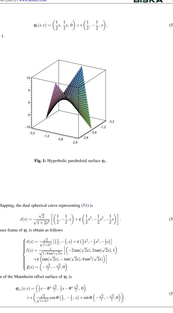
ϕe(s,v) =
( 1 2s,
1 2s,0
) +v
( 1 2,−
1 2,s
)
, (51)
and rendered in Fig. 1.
Fig. 1:Hyperbolic paraboloid surfaceϕe.
From the E. Study Mapping, the dual spherical curve representing (51) is
˜
e(s) =
√
2
√
1+2s2 [(
1 2,−
1 2,s
) +ε ( 1 2s 2, −1 2s 2, −1 2s )] . (52)
Then, the dual Darboux frame ofϕeis obtain as follows
˜
e(s) =√√2 1+2s2
[(1 2,−
1 2,s
) +ε(1
2s 2,−1
2s 2,−1
2s )]
˜
t(s) =√ 1 1+8 tan2(√2s)
[(
−2 tan(√2s),2 tan(√2s),1)
+ε(tan(√2s),−tan(√2s),4 tan2(√2s))] ˜
g(s) =(−√22,−
√
2 2 ,0
)
The general equation of the Mannheim offset surface ofϕeis
ϕe1(s,v) =
( 1 2s−θ∗
√
2 2 ,
1 2s−θ∗
√
2 2 ,0
)
+v
( √
2
√
1+2s2cosθ
(1 2,−
1 2,s
)
+sinθ(−√22,−
√
2 2 ,0
))
Fig. 2:Mannheim offsetϕe1with dual offset angle ¯θ=0+ε4
√
2.
Fig. 3:Mannheim offsetϕe1 with dual offset angle ¯θ=π/4+ε2
√
2.
From (53) we can give the following special cases:
i)The Mannheim offsetϕe1with dual offset angle ¯θ=0+ε4
√
2 is
ϕe1(s,v) =
( 1 2s−4,
1 2s−4,0
) +v
( √
2
√
1+2s2,−
√
2
√
1+2s2,
√
2s √
1+2s2 )
which is an oriented offset ofϕe(Fig. 2).
ii)The Mannheim offsetϕe1 with dual offset angle ¯θ=π/4+ε2
√
ϕe1(s,v) =
( 1 2s−2,
1 2s−2,0
) +v
( 1 2√1+2s2−
1 2,
−1 2√1+2s2−
1 2,
s √
1+2s2 )
4 Conclusions
In the surface theory, offset surfaces have an important role and large applications in many areas. Especially, the ruled surface offsets are interesting since these surfaces can be generated by a continuous moving of a straight line. In this paper, some new results including the characterizations of Mannheim surface offsets have been obtained in dual space. Furthermore, the relationships for Mannheim surface offsets to be developable have been introduced.
References
[1] Blaschke, W., Vorlesungen uber Differential Geometrie, Bd 1, Dover Publ., New York, (1945).
[2] Dimentberg, F. M., The Screw Calculus and its Applications in Mechanics, (Izdat. Nauka, Moscow, USSR, 1965) English translation: AD680993, Clearinghouse for Federal and Scientific Technical Information.
[3] Hacısalihoˇglu. H.H., Hareket Gometrisi ve Kuaterniyonlar Teorisi, Gazi ¨Universitesi Fen-Edb. Fak¨ultesi, (1983). [4] Hoschek, J., Lasser, D., Fundamentals of computer aided geometric design, Wellesley, MA:AK Peters; 1993.
[5] Karger, A., Novak, J., Space Kinematics and Lie Groups, STNL Publishers of Technical Lit., Prague, Czechoslovakia (1978). [6] K¨uc¸¨uk, A., G¨ursoy O., On the invariants of Bertrand trajectory surface offsets, App. Math. and Comp., 151 (2004) 763-773. [7] Orbay, K., Kasap, E., Aydemir, ˙I, Mannheim Offsets of Ruled Surfaces, Mathematical Problems in Engineering, Volume 2009,
Article ID 160917.
[8] ¨Onder, M., Uˇgurlu, H.H., On the Developable of Mannheim offsets of spacelike ruled surfaces, arXiv:0906.4660v4 [math.DG]. [9] ¨Onder, M., Uˇgurlu, H.H., On the Developable of Mannheim offsets of timelike ruled surfaces in Minkowski 3-space, Proc. Natl.
Acad. Sci., India, Sect. A Phys. Sci., 84(4) (2014) 541-548.
[10] ¨Onder, M., Uˇgurlu, H.H., Some Results and Characterizations for Mannheim Offsets of Ruled Surfaces, Bol. Soc. Paran. Mat. 34(1) (2016) 85-98.
[11] Papaioannou, S.G., Kiritsis, D., An application of Bertrand curves and surfaces to CAD/CAM, Computer Aided Design 17(8) (1985) 348-352.
[12] Pottmann, H., L¨u, W., Ravani, B., Rational ruled surfaces and their offsets, Graphical Models and Image Processing, 58(6) (1996) 544-552.
[13] Ravani, B., Ku, T.S., Bertrand Offsets of ruled and developable surfaces, Comp. Aided Geom. Design, 23(2) (1991) 147-152. [14] Veldkamp, G.R., On the use of dual numbers, vectors and matrices in instantaneous spatial kinematics, Mechanism and Machine