ISSN 0101-8205 www.scielo.br/cam
Successive linear approximation for finite elasticity
I-SHIH LIU, ROLCI A. CIPOLATTI and MAURO A. RINCON
Instituto de Matemática, Universidade Federal do Rio de Janeiro 21945-970 Rio de Janeiro, RJ, Brasil
E-mails: [email protected] / [email protected] / [email protected]
Abstract. A method of successive Lagrangian formulation of linear approximation for solving boundary value problems of large deformation in finite elasticity is proposed. Instead of solving the nonlinear problem, by assuming time steps small enough and the reference configuration updated at every step, we can linearize the constitutive equation and reduce it to linear boundary value problems to be solved successively with incremental boundary data. Moreover, nearly incompressible elastic body is considered as an approximation to account for the condition of incompressibility. For the proposed method, numerical computations of pure shear of a square block for Mooney-Rivlin material are considered and the results are compared with the exact solutions.
Mathematical subject classification: Primary: 65C20; Secondary: 74B20.
Key words: large deformation, nonlinear elastic materials, successive Lagrangian formula-tion, boundary value problem, incremental method, numerical computation.
1 Introduction
The constitutive equation of a solid body is usually expressed relative to a pre-ferred reference configuration which exhibits specific material symmetries such as isotropy. The constitutive functions are generally nonlinear. Therefore, for large deformations, it leads to a system of nonlinear partial different equations for the solution of boundary value problems. The problems are usually formu-lated in Lagrangian coordinates in the preferred reference configuration, and
numerical methods involve solving nonlinear systems as well as having other difficulties, such as the boundary conditions may involve the deformed state which depends on the solutions themselves. Alternatively, we are proposing a different method for solving boundary value problem of large deformation in a successive Lagrangian formulation of linear approximation.
Roughly speaking, the method of successive linear approximation is similar to the Euler method for solving differential equations, i.e., successively at each state, the tangent is calculated and projected to a neighboring state. In other words, the constitutive equations are calculated at each state which will be re-garded as the reference configuration (updated Lagrangian formulation) for the next state, and assuming the deformation to the next state is small, the updated constitutive equations are linearized. In this manner, it becomes a linear problem just like the problems in linear elasticity from one state to the next state with incremental small deformations.
For numerical computation of large deformations, “incremental methods” have been widely discussed ([4, 7, 6]). The problems are usually formulated with domains in the initial reference configuration, i.e., in “total” Lagrangian formulation. This is the essential difference from the method proposed in this paper in which at each step the reference configuration is updated in the “succes-sive” Lagrangian formulation. Although the two approaches are mathematically equivalent, the basic equations and numerical treatment of boundary conditions are quite different. From the examples of pure shear, some advantages of the present approach are discussed.
2 Updated reference configuration
Letκr be the preferred reference configuration of an elastic bodyB, and
x =χ (X,t), X ∈κr(B),
be the deformation of the bodyκr(B)at timet. LetF(X,t)be the deformation gradient and the Cauchy stressT(X,t)be given by the constitutive equation
It is well-known that the constitutive model based on the linear constitutive equation, Hooke’s law, does not satisfy the principle of material frame-indif-ference, and it can only be regarded as an approximation of some nonlinear model for small deformations (see [3, 2]). Therefore, in order to consider large deformations, the constitutive functionFκr is generally a nonlinear function of
the deformationF.
Letκt0 be the deformed configuration at timet0. The deformation
ξ =χ (X,t0)
fromκr toκt0 need not be small. Let
F0= F(X,t0)= ∇Xξ, T0=T(X,t0),
be the deformation gradient with respect to configuration κr and the Cauchy stress att0respectively.
Now, consider a deformation fromκt0 to the configurationκt at time t > t0
such that the displacement vector
u=χ (X,t)−ξ, H = ∇ξu,
where H is the displacement gradient with respect to the updated reference configurationκt0 (emphasize, notκr). Then
F =F(X,t)= ∇Xξ + ∇ξu∇Xξ,
or
F =(I +H)F0.
Therefore, we can represent the deformation and deformation gradient schemat-ically in the following diagram:
F0 I +H
X ∈κr(B) −−−−−−→ ξ ∈κt0(B) −−−−−−→ x ∈κt(B)
ξ =χ (X,t0) x =ξ+u
2.1 Linearized constitutive equations
We shall assume that the displacement gradient H is small, |H| ≪ 1, and linearize the constitutive equation (1) relative to the configurationκt0, namely,
T =T0+ ∇FFκr(F0)[F −F0] =T0+ ∇FFκr(F0)[H F0],
or
T =T0+L(F0)[H], (3)
where
L(F0)[H] = ∇FFκr(F0)[H F0] (4)
defines the fourth order elasticity tensorL(F0)relative to the reference configu-rationκt0.
Furthermore, the (first) Piola-Kirchhoff stress tensor relative to the updated reference configurationκt0 is given by
Tκt0 =det(I +H)T(I +H)
−T
=det(I +H) T0+L(F0)[H](I +H)−T
=(I +trH) T0+L(F0)[H]
(I −HT)+o(2)
=T0+(trH)T0−T0HT +L(F0)[H] +o(2),
whereo(2)represents higher order terms in the small displacement gradient|H|. We can also define the elasticity tensor for the Piola-Kirchhoff stress by
Lκt0(F0,T0)[H] =(trH)T0−T0H
T +L(F0)[H], (5)
and write the linearized Piola-Kirchhoff stress as
Tκt0 =T0+Lκt0(F0,T0)[H]. (6)
2.2 Nearly incompressible elastic body
For an incompressible elastic body, the constitutive equation (1) should be replaced by
where pdenotes the pressure which theoretically for a (perfectly) incompress-ible material body depends not only on the deformation of the body, but also on the boundary conditions.
However, we shall consider only nearly incompressible bodies, and assume that the pressure is a function of density,p = p(ρ), or inversely, the density is a function of pressure,ρ =ρ(p). Therefore, bynearly incompressiblewe mean that the density is nearly insensitive to the change of pressure, i.e., the densityρ is nearly constant, i.e.,
dρ
d p ≈const.≪1. (8)
In the approximation considered in (2), since F = (I + H)F0, the Cauchy stress in the configurationsκt andκt0 are given by
T = −p I +Fκr(F), T0= −p0I +Fκr(F0),
Linearization inH with (4) gives
T −T0= −(p− p0)I + ∇FFκr(F0)[H F0] = −(p−p0)I +L(F0)[H]. (9)
On the other hand, from the equation of mass balance, we have
˙
ρ+ρdivx˙ =0,
and sinceρ =ρ(p), it follows that
˙
p+βtr gradx˙ =0, (10)
where
β =ρ
dρ
d p
−1
≫1 (11)
is a time-independent constant, much greater than 1, by the assumption (8). Furthermore, since gradx˙ = ˙F F−1and F = (I +H)F0, by assuming also that| ˙H| ≪1, we have
gradx˙ = ˙H F0((I +H)F0)−1= ˙H F0F0−1(I −H)+o(2)= ˙H+o(2), and the equation (10) becomes
˙
which by integration leads to
p−p0= −βtrH.
Consequently, from (9), the Cauchy stress becomes
T =T0+β(trH)I +L(F0)[H], (12)
and from (6), the Piola Kirchhoff stress
Tκt0 =T0+β(trH)I +Lκt0(F0,T0)[H]. (13)
Remark. Perhaps, someone might regard the parameterβ introduced in (11) as a penalization parameter. However, it is different from the usual penaliza-tion method which introduces a penalizing term into the momentum equapenaliza-tion to account for kinematical or geometrical restrictions. In the present context, it is a consequence of near-incompressibility assumption (8) resulting in the elim-ination of the pressure from the constitutive equation by integrating the mass balance equation, and there is no need to modify the momentum equation.
2.3 Mooney-Rivlin materials
As an example, we shall consider a (nearly) incompressible Mooney-Rivlin ma-terial with the constitutive equation given by
T = −p I +Fκr(F), Fκr(F)=s1B+s2B
−1
, (14)
whereB = F FT is the left Cauchy-Green strain tensor and the coefficients are constants.
From (4) and (5), after taking the gradient ofFκr(F)atF0, we have
L(F0)[H] =s1(H B0+B0HT)−s2(B0−1H+HTB0−1), and
Lκt0(F0,T0)[H] =(trH)T0−T0H
T +s1(H B0+B0HT)
−s2(B0−1H+HTB0−1).
3 Linearized boundary value problem
We can now consider the updated Lagrangian formulation of the boundary value problem. Let = κ(B) ⊂ IR3 be the region occupied by the body at the configurationκ (standing forκt0 and instead ofξ, useX as a typical point of
κ(B)for simplicity). ∂=Ŵ1∪Ŵ2, andnκ be the exterior unit normal to∂.
Let the displacement vector relative to the configurationκbe
u(X,t)=x(X,t)−X, x(X,t0)=X.
Consider the boundary value problem of an elastic body in equilibrium without external body force given by
−DivTκ =0 in ,
Tκnκ = f on Ŵ1,
u= g on Ŵ2,
(15)
where the surface traction f(X,t0)and the displacementg(X,t0)are prescribed. Assuming that att0, the deformation gradientF0with respect to the preferred configurationκr and the Cauchy stress T0are known, and that1t = t−t0 is small enough, then from (13), we have
Tκ =T0+β(trH)I +Lκt0(F0,T0)[H] :=T0+ ˜Lκ(F0,T0)[H], (16)
whereH(X,t)= ∇u(X,t)is the displacement gradient with respect toXin the configurationκ. Upon substitution into (15), we have the following problem:
−Div(L˜κ(F0,T0)[∇u])=DivT0 in ,
(L˜κ(F0,T0)[∇u])nκ = f −T0nκ on Ŵ1,
u= g on Ŵ2.
(17)
At every time step, the idea of formulating the boundary value problem in the form (17) is similar to the theory of small deformations superposed on finite deformations (see [2, 1]). In this manner, either we are interested in the evolu-tion of soluevolu-tions with gradually changing boundary condievolu-tions resulting in large deformation, or, we can treat the boundary values of finite elasticity as the final value of a successive small incremental boundary values at each time step.
Remark 3.1. The constantβwill be taken as a constant large enough to guaran-tee the near-incompressibility, which in numerical computation can be checked from the condition detF ≈1.
4 Numerical solution for large deformations
Recall the Euler method of solving differential equation, say y˙ = f(t), that for a discrete time axis,∙ ∙ ∙<tn−1<tn <tn+1<∙ ∙ ∙, andy(tn)=yn, the solution curve can be constructed byyn+1=yn+ f(tn)1t, where f(tn)is the tangent of the solution curve attn. We can use a similar strategy for solving problems of large deformation, by solving linear boundary value problem stated in (17).
We consider a discrete time axis,∙ ∙ ∙ < tn−1 < tn < tn+1 < ∙ ∙ ∙ with small enough constant spacing 1t. Let κtn be the configuration of the body at the
instanttnand
X =x(X,tn)∈κtn(B).
Let
F0=F0(X,tn), T0=T0(X,tn)
be the deformation gradient relative to the preferred configuration κr and the Cauchy stress respectively. The boundary value problem (17) with boundary data f(X,tn)andg(X,tn)in Lagrangian formulation with respect to the refer-ence configurationκtn, can now be solved as a problem in linear elasticity for
the displacement fieldu(X,tn+1)from the configurationκtn.
After solving the problem (17) at tn, the reference configurationκtn+1 attn+1
can be updated from the displacement field, i.e.,
while the deformation gradient
F0(X,tn+1)=(I +H(X,tn+1))F0(X,tn)
and the Cauchy stress from (10)
T0(X,tn+1)=T0(X,tn)+βtrH(X,tn+1)I +L(F0(X,tn))H(X,tn+1)
can be calculated attn+1 so that the Lagrangian formulation of the problem in the form (17), with boundary data f(X,tn+1)andg(X,tn+1), can proceed again from the updated reference configuration attn+1. This numerical procedure will be referred to as thesuccessive Lagrangian formulation of linear approximation for large deformations, or simply as the method ofSuccessive Linear Approxi-mation(SLA).
Boundary value problems in finite elasticity known as Ericksen’s problem are the textbook examples for which the exact solutions can be obtained by apply-ing suitable surface tractions on the boundary alone irrespective of constitutive properties of the elastic bodies. Such controllable deformations are called uni-versal solutions, and for any incompressible isotropic elastic bodies, there are several known classes of problems including homogeneous deformation, shear-ing, bendshear-ing, torsion, inflation and eversion [3, 2]. In developing a numerical method for large deformations, such problems with exact solutions can be used as benchmark problems for comparison. In the following we shall consider one such problem: pure shear of a square block.
5 Example: pure shear
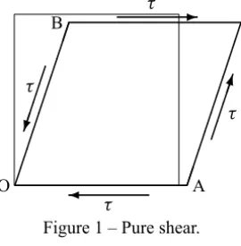
For applying the method of SLA, we consider the case of pure shear of a square block, by applying tangential surface traction, the shear stressτ, on the surface of the block as shown in Figure 1.
τ
τ
τ τ
O A
B
Figure 1 – Pure shear.
5.1 Exact solution
Theoretically, the shear deformation can be described as
x1=λ1X1+κλ2X2, x2=λ2X2, x3=λ3X3. (18)
In the case of pure shear, for which there are no applied normal stresses on the surface, it can be proved (see for example, [3, 5]) that for any elastic material body, the deformed state of a square block maintains the geometric shape of an equilateral parallelogram as shown in Figure 1, i.e.,
O A=O B, or λ21= 1+κ 2
λ22. (19)
Furthermore, for Mooney-Rivlin materials, from (14) and (18), the shear stress τ =T12 is given by
τ =κ s1λ22−s2λ−21 . (20) In the following numerical computation, we shall consider the two-dimen-sional case, so that the thickness inx3-direction remains unchanged, i.e.,
λ3=1, and λ1λ2=1,
by incompressibility. Consequently, from (19) and (20), it follows that
λ1= 1−τ2(s1−s2)−2−1/4, κ = λ41−1
1/2
. (21)
5.2 Numerical results
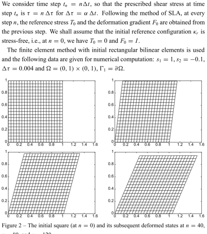
We consider time step tn = n1t, so that the prescribed shear stress at time steptn isτ = n1τ for1τ = α 1t. Following the method of SLA, at every stepn, the reference stressT0and the deformation gradientF0are obtained from the previous step. We shall assume that the initial reference configurationκr is stress-free, i.e., atn =0, we haveT0=0 andF0=I.
The finite element method with initial rectangular bilinear elements is used and the following data are given for numerical computation:s1=1,s2= −0.1, 1τ =0.004 and=(0,1)×(0,1),Ŵ1=∂.
0 0.2 0.4 0.6 0.8 1
0 0.2 0.4 0.6 0.8 1 1.2 1.4 1.6 0 0.2 0.4 0.6 0.8 1
0 0.2 0.4 0.6 0.8 1 1.2 1.4 1.6
0 0.2 0.4 0.6 0.8 1
0 0.2 0.4 0.6 0.8 1 1.2 1.4 1.6 0 0.2 0.4 0.6 0.8 1
0 0.2 0.4 0.6 0.8 1 1.2 1.4 1.6
Figure 2 – The initial square (atn =0) and its subsequent deformed states atn =40,
n=80, andn=120.
by comparing the consecutive sides of the parallelogram,(0A−0B)/0A, using a mesh of 20×20 elements.
The deformation given by (18) is homogeneous, and the figures in Figure 2 seem to confirm this. In other words, theoretically the deformation gradientFis constant. In particular, so are the values ofλ1=F11and detF. These values have been checked, and surely, they are not expected to be exactly constant everywhere in the numerical results. Instead, we shall see how good those values are from being constant by showing their average values together with their minima and maxima over the body in Table 1 and Table 2.
n λex1 λav1 λmin1 –λmax1 Average Error 40 1.005360 1.005195 (1.003931 – 1.006040) 0.0164% 80 1.022352 1.022929 (1.020991 – 1.024568) 0.0564% 120 1.054227 1.060329 (1.056625 – 1.062738) 0.5788%
Table 1 – Comparison of the exact value ofλ1with the values obtained from numerical results at various stepn.
n Jav Jmin–Jmax
40 1.000000 (0.999994 – 1.000001) 80 0.999996 (0.999988 – 0.999999) 120 0.999969 (0.999955 – 0.999976)
Table 2 – Verification of the incompressibility conditionJ=detF≈1 in the numerical simula-tion at various stepn.
At step n, the exact value of λ1, given in Table 1, is calculated from the equation (21) for the shear stressτ =n1τ. The corresponding value obtained from the numerical computation is shown in the table. From the average value over the body and the percentage error,|λav1 −λex1|/λex1 , it shows that it is in very good agreement with the analytical prediction. In addition, to show the value is nearly constant in the body, the minimum and the maximum values ofλ1are also given.
6 Final remarks
For numerical computation of large deformations in finite elasticity, to obviate the difficulty of handling nonlinearities, “incremental methods” are widely dis-cussed, for example, in the books by Oden [4], Ogden [7] and Ciarlet [6]. These methods consist in letting the boundary forces vary by small increments from zero to the given ones and to compute corresponding approximate solutions by successive linearization. The general idea seems to be of purely mathematical concern regarding linearization between successive boundary value problems. The problems are usually formulated with domains in the initial reference con-figuration, i.e., in Lagrangian formulation.
From mathematical viewpoint, the basic idea of the present method (SLA) is similar to the other incremental methods, except that it is formulated using the current state as the reference configuration and not relying on the incremental loading as the driving force for further deformations. Consequently, it would be possible to prove existence and uniqueness of successive incremental solu-tions with proper regularity condisolu-tions on the current state of the body (see for example [6]).
The conceptually simpler approach of the present method with successively updated Lagrangian formulation at each step is mainly motivated from phys-ical viewpoint. It also has an advantage that the prescription of (incremental) boundary data is simpler and straightforward, if we remember that in Lagrangian formulation, the corresponding boundary tractions to be prescribed in the ini-tial reference configuration generally depend on the surface geometry of the deformed configuration.
Therefore, the difference between applying the corresponding tractions on the surfaces of the consecutive states is of higher orders which is insignificant in the linear approximation.
Another advantage of this formulation for (nearly) incompressible elastic body lies in the elimination of the pressure from the integration of the equation of mass balance. This is possible due to the assumption of near-incompressibility, so that unlike the usual formulation there is no need to consider the pressure as an unknown variable in addition to the unknown displacement vector function.
Acknowledgements. The authors (ISL and MAR) are partially supported by CNPq-Brasil.
REFERENCES
[1] A.E. Green, R.S. Rivlin and R.T. Shield, General theory of small elastic deformations superposed on finite deformations. Pro. Roy. Soc. London, Ser. A,211(1952), 128–154.
[2] C. Truesdell and W. Noll, The Non-Linear Field Theories of Mechanics. 3rd edition. Springer: Berlin (2004).
[3] I-S. Liu,Continuum Mechanics. Springer: Berlin Heidelberg (2002).
[4] J.T. Oden. Finte Elements of Nonlinear Continua. McGraw-Hill, New York (1972).
[5] K.R. Rajagobal and A.S. Wineman, New universal relations for nonlinear isotropic elastic materials. J. Elasticity,17(1987), 75–83.
[6] P.G. Ciarlet, Mathematical Elasticity. Three-Dimensional Elasticity, 1, North-Holland, Amsterdam (1988).