FACULDADE DE ECONOMIA, ADMINISTRAÇÃO, ATÚARIA E CONTABILIDADE PROGRAMA DE PÓS-GRADUAÇÃO EM ECONOMIA - CAEN
DIEGO DE MARIA ANDRÉ
THREE ESSAYS ON APPLIED MICROECONOMETRICS WITH SPATIAL EFFECTS
THREE ESSAYS ON APPLIED MICROECONOMETRICS WITH SPATIAL EFFECTS
Tese de Doutorado submetida à Coordenação do Programa de Pós-Graduação em Economia – CAEN, da Faculdade de Economia, Adminis-tração, Atúaria e Contabilidade da Universi-dade Federal do Ceará, como requisito parcial para a obtenção do título de Doutor em Ci-ências Econômicas. Área de concentração: Econometria aplicada.
Prof. Dr. José Raimundo de Araújo Carvalho Júnior
Gerada automaticamente pelo módulo Catalog, mediante os dados fornecidos pelo(a) autor(a)
A573t André, Diego de Maria.
Three essays on applied microeconometrics with spatial effects / Diego de Maria André. – 2016. 95 f. : il. color.
Tese (doutorado) – Universidade Federal do Ceará, Faculdade de Economia, Administração, Atuária e Contabilidade, Programa de Pós-Graduação em Economia, Fortaleza, 2016.
Orientação: Prof. Dr. José Raimundo de Araújo Carvalho Júnior.
1. Microeconometria. 2. Econometria espacial. I. Título.
Tese de Doutorado submetida à Coordenação do Programa de Pós-Graduação em Economia – CAEN, da Faculdade de Economia, Adminis-tração, Atúaria e Contabilidade da Universi-dade Federal do Ceará, como requisito parcial para a obtenção do título de Doutor em Ci-ências Econômicas. Área de concentração: Econometria aplicada.
Aprovada em: 18 de Maio de 2016.
BANCA EXAMINADORA
Prof. Dr. José Raimundo de Araújo Carvalho Júnior (Orientador)
Universidade Federal do Ceará (UFC)
Prof. Dr. João Mário Santos de França Universidade Federal do Ceará (UFC)
Prof. Dr. Emerson Luís Lemos Marinho Universidade Federal do Ceará (UFC)
Prof. Dr. Victor Hugo de Oliveira Silva Instituto de Pesquisa e Estratégia Econômica do
Ceará (IPECE)
Prof. Dr. Cleyber Nascimento de Medeiros Instituto de Pesquisa e Estratégia Econômica do
Nesse momento tão especial da minha vida, não poderia deixar de agradecer as pessoas que de alguma forma contribuiram para que eu alcançasse o meu objetivo. Em primeiro lugar, agradeço a Deus, por nos dar a oportunidade de vivenciar esse grande mistério que é a vida.
Agradeço aos meus pais, Haroldo e Célia, que através de muito esforço e dedicação, conseguiram me dar educação e me ensinaram a valorizar as pequenas coisas da vida, mostrando-me que só tem valor aquilo que é conseguido com o suor do nosso trabalho. Se hoje sou Doutor em economia, devo isso eles. Obrigado!
A minha esposa, Talita, que durante os nossos quase 9 anos juntos, sempre tem me dado apoio, amor e carinho nos momentos díficeis, sempre me incentivando a continuar a busca por soluções quando estou quase desistindo. Sem esses incentivos, com certeza, não teria conseguido. Te amo e Obrigado!
Ao professor José Raimundo, com quem tenho aprendido bastante nesses 6 anos em que temos trabalhado juntos (Mestrado e Doutorado), e cujos ensinamentos levarei para a vida toda.
Aos professores João Mário, Emerson Marinho, Victor Hugo e Cleyber Nasci-mento por disponibilizarem seu tempo para participar da banca de avaliação e por suas contribuições ao trabalho.
Aos demais professores do CAEN por suas contribuições à minha formação acadê-mica.
A todos os funcionários do CAEN, em especial ao Cléber e o S. Adelino, que com suas conversas e brincadeiras ajudam a tornar o CAEN um lugar especial.
Agradeço ainda à todos os colegas do Laboratório de Econometria e Otimização (LECO), não só os atuais (Sylvia, Abel, Luan, Marcelino, Sara) mas a todos os que em algum momento passaram pelo LECO durante os 6 anos que trabalho lá (Luis Carlos, Yuri, Isadora), pelo convívio e trocas de conhecimento e experiências. Agradeço também a todos os colegas de Mestrado e Doutorado do CAEN.
Por fim, agradeço ao CAEN por disponibilizar sua estrutura para a realização deste trabalho e a CAPES pela bolsa concedida.
A presente tese é composta por três capítulos, independentes entre si, em microeconometria aplicada. O primeiro capítulo aplica o instrumental teórico e empírico da econometria espacial para analisar os determinantes da demanda residencial de água para a cidade de Fortaleza (Brasil). Estimamos três modelos econométricos, que tem como variáveis explicativas o preço médio/marginal, a diferença, renda, número de homens e mulheres residentes, número de banheiros, sob diferentes especificações espaciais: O modelo de erro espacial (SEM), o modelo espacial autorregressivo (SAR) e o modelo espacial autorregressivo de médias móveis (SARMA), sendo o modelo SARMA o que melhor se ajusta aos dados. Os resultados indicaram que não controlar pelos efeitos espaciais é uma fonte de erro de especificação, subestimando o efeito de quase todas as variáveis. Algumas vezes, essas diferenças podem chegar a 24.66% e 13.32% para a elasticidade-preço no modelo de preço médio e no modelo de McFadden, respectivamente. No segundo capítulo estima-se a disposição a pagar (WTP) pela redução estocástica de primeira ordem no risco de ser roubado, para a cidade de Fortaleza (Brasil). Inspirado por Cameron e DeShazo (2013), desenvolveu-se um modelo simples de escolha que aninha o processo de avaliação contingente (CV) entre loterias e estimou-se por máxima verossimilhança paramétrica e pelo modelo de regressão geograficamente ponderada (GWR). Para o modelo global, isto é, sem efeitos espaciais, estimou-se uma disposição a pagar média de R$ 23.35 por mês/por residência, e um valor implícito de um roubo estatístico de R$ 11,969 por crime evitado. Para o modelo local (GWR), implementou-se o protocolo da krigagem para calcular uma superfície de disposição a pagar. Os resultados sugerem que embora na periferia a disposição a pagar seja menor, à medida que vamos para o centro da cidade existe muita heterogeneidade na distribuição espacial da disposição a pagar para a redução do risco de roubo. No terceiro capítulo analisou-se como o rendimento acadêmico de alunos universitários é afetado pelos seus colegas de sala, através de um desenho descontínuo. Utilizando dados da Universidade Federal do Ceará (UFC), empregamos o modelo de regressão descontínua (RDD) para estimar a diferença entre entrar na turma do primeiro ou do segundo semestre. Devido à quantidade de cursos disponível na nossa base de dados, classificamos os cursos em quatro categorias, de acordo com as notas de entrada no vestibular. Então, procedemos com a estimação de um modelo multi-tratamento. Os resultados mostram que os alunos que foram classificados um pouco acima do limite de vagas (turma do primeiro semestre) têm rendimento acadêmico 2% menor (-0.19) do que alunos que tiveram classificação um pouco abaixo desse limite (turma do segundo semestre). Ademais, encontramos não linearidades nesses efeitos, assim como Sacerdote (2001) e Zimmerman (2003), com intervalos entre 2.5 e -0.18.
Palavras-chave: Demanda por água. Efeitos Espaciais. Crime. Avaliação Contingente.
This Thesis consists of three independent essays on applied microeconometrics. The first chapter applies theoretical and empirical tools of spatial econometrics to analyze the deter-minants of residential water demand function for the city of Fortaleza (Brazil). We estimated three econometric models, which have as explanatory variables the average/marginal price, the difference, income, number of male and female residents and the number of bathrooms, under different spatial specifications: the Spatial Error Model (SEM), the Spatial Auto-regressive model (SAR), and finally, the Spatial AutoAuto-regressive Moving Average model (SARMA), which is the model that best fitted the data. Results suggest that not control-ling for spatial effects is a key specification error, underestimating the effect of almost all variables in the model. Sometimes, these differences can be as high as 24.66 % and 13.32 % for price elasticity in the Average Price and the McFadden models, respectively. In the second chapter we estimated willingness to pay (WTP) for a first order stochastic reduction on the risk of robbery, for the city of Fortaleza (Brazil). Inspired by Cameron and DeShazo (2013), we develop a simple choice model that nests a process of contingent valuation (CV) among lotteries and estimate it by both parametric maximum likelihood and geographically weighted regression (GWR). For the global model (i.e., without spatial effects), we estimated an average WTP of R$ 23.35 per month/household, and an implicit value of a statistical robbery approximately equal to R$ 11,969 per crime avoided. For the local model (GWR), we implement a protocol to calculate a surface of WTP using Kriging techniques. The results suggests that although peripheries present lower willingness to pay, as long as we go inwards there is plenty of heterogeneity on its spatial distribution for risk reductions. In the third chapter we analyzed how undergraduate students’ academic performance is affected by theirs classmates, by means of a “discontinuity design”. With data from Ceará Federal University (UFC), we employed regression discontinuity design (RDD) to estimate the difference between entering in the first semester class or second semester class. Due to the great courses availability, we assign each course into one of four categories depending on its admitted students’ results at the entrance exam. Then, we proceed the estimation exercise using a multi-treatment effect model. Results show that students who were ranked just above the cutoff (first semester class) had an academic performance 2% smaller (-0.19) than students who were ranked just below the cutoff (se-cond semester class). Moreover, we found non-linearities in this effect, as well as Sacerdote (2001) and Zimmerman (2003), with intervals between 0.5 to -0.18.
Figure 1.1 – Geographical location of the city of Fortaleza . . . 11
Figure 3.1 – Survival Function . . . 39
Figure 3.2 – First-Order Stochastic Dominance . . . 41
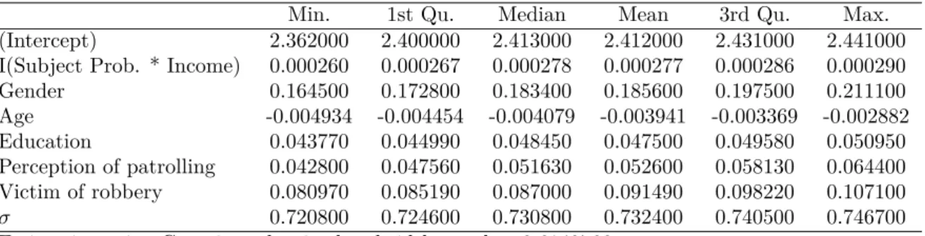
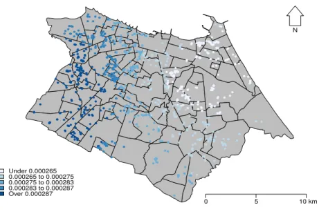
Figure 3.3 – Estimated parameters of spatial distribution - Subject Prob. * Income 49 Figure 3.4 – Estimated parameters of spatial distribution - Gender . . . 49
Figure 3.5 – Estimated parameters of spatial distribution - Age . . . 50
Figure 3.6 – Estimated parameters of spatial distribution - Education . . . 50
Figure 3.7 – Estimated parameters of spatial distribution - Perception of patrolling . 51 Figure 3.8 – Estimated parameters of spatial distribution - Victim of robbery . . . . 51
Figure 3.9 – Willingness to Pay - Spatial Distribution . . . 52
Figure 3.10–Willingness to Pay - Kriging Surface . . . 53
Figure 4.1 – Distribution of normalized assignment grade by courses - Medical school and Law school . . . 67
Figure 4.2 – Distribution of normalized assignment grade by courses - College of Economics, Management, Actuarial Science and Accounting . . . 68
Figure 4.3 – Distribution of normalized assignment grade by courses - College of Sciences and College of Agricultural Sciences . . . 69
Figure 4.4 – Distribution of normalized assignment grade by courses - College of Humanities . . . 70
Figure 4.5 – Distribution of normalized assignment grade by courses . . . 71
Figure 4.6 – IRA results as a function of standard assignment grade . . . 76
Figure 4.7 – Sensitivity test . . . 77
Figure 4.8 – McCrary test . . . 78
Table 2.1 – Descriptive Statistics . . . 17
Table 2.2 – Estimates Average Price, Marginal Price and Mc Fadden, No Spatial Effects . . . 23
Table 2.3 – Estimates Average Price and McFadden, with Spatial Effects . . . 25
Table 2.4 – Total Impact on AP and McFadden Models . . . 25
Table 2.5 – Percentual Variation (%) - 100× βbT otalSpatial−βbN onSpatial b βN onSpatial . . . 26
Table 3.1 – Variables’ descriptions . . . 36
Table 3.2 – Sample Description - Total . . . 37
Table 3.3 – Sample description - Protesters . . . 38
Table 3.4 – Sample description - Willing to Pay . . . 38
Table 3.5 – Willingness to pay frequency distribution . . . 38
Table 3.6 – Estimates - Parametric Maximum Likelihood . . . 47
Table 3.7 – Results of WTP(R$) from the global parametric model . . . 47
Table 3.8 – Estimates for the Local Model - GWR -Adaptive bandwidth . . . 48
Table 4.1 – Variables descriptions . . . 65
Table 4.2 – Descriptive statistics . . . 65
Table 4.3 – Definitions of treatments groups . . . 72
Table 4.4 – SRD estimates for the effect of being in the first semester class on students’ IRA . . . 75
Table 4.5 – Effects of policies in some studies . . . 76
Table 4.6 – Covariates balanced test . . . 78
Table 4.7 – SRD estimates for the effect of being in the first semester class on students’ IRA — Multi-treatment . . . 79
Table 4.8 – Incremental and comparison with the control effects . . . 81
Table 4.9 – SRD estimates for the effect of being in the first semester class on students’ IRA — Classified by areas of knowledge . . . 87
Table 4.10–SRD estimates for the effect of being in the first semester class on students’ IRA — Divided by semesters . . . 88
1 GENERAL INTRODUCTION . . . 11
2 SPATIAL DETERMINANTS OF URBAN RESIDENTIAL WATER DEMAND IN FORTALEZA, BRAZIL . . . 14
2.1 Introduction . . . 14
2.2 Water Micro Demand Estimation with Spatial Effects . . . 15
2.3 Data Set . . . 16
2.3.1 The Sample . . . 16
2.3.2 Spatial Exploratory Data Analysis . . . 17
2.4 Econometric Model . . . 18
2.4.1 Non-Spatial Specification . . . 18
2.4.2 Spatial Specification . . . 20
2.4.3 Why Spatial Effects in Water Demand? . . . 21
2.5 Results . . . 22
2.5.1 Non-Spatial Specification . . . 22
2.5.2 Spatial Specification . . . 24
2.6 Final Considerations . . . 26
References . . . 28
3 SPATIAL WILLINGNESS TO PAY FOR A FIRST-ORDER STOCHAS-TIC REDUCTION ON THE RISK OF ROBBERY . . . 31
3.1 Introduction . . . 31
3.2 Data Set . . . 35
3.3 Econometric Model . . . 39
3.4 A “Local” Econometric Model . . . 44
3.5 Results . . . 46
3.5.1 Results from the Global Model . . . 46
3.5.2 Results from the Local Model . . . 48
3.6 Final Considerations . . . 53
References . . . 55
4 PEER EFFECTS AND ACADEMIC PERFORMANCE IN HIGHER EDUCATION - A REGRESSION DISCONTINUITY DESIGN AP-PROACH . . . 57
4.2.2 The use of regression discontinuity design . . . 60
4.3 The entrance process in Brazilian universities . . . 62
4.4 Data . . . 63
4.5 Empirical strategy . . . 72
4.6 Results . . . 75
4.7 Final Considerations . . . 81
This Thesis is a collection of three independent essays on microeconometrics using data from the city of Fortaleza (Brazil). In the first chapter, I examine the determinants of urban residential water demand. The second chapter studies willingness to pay for a reduction on the risk of robbery. The third chapter studies how “peer effects” determines academic performance in high education.
Fortaleza is the state capital of Ceará. Located in northeastern Brazil, a dry climate region, the city has a population of about to 2.5 million and it is the fifth largest city in Brazil with an area of 313 square kilometers, boasting one of the highest demographic
densities in the country (8,001 per km2). Fortaleza’s economy is mainly based on trade,
service, and tourism and its gross domestic product is the largest in northeastern Brazil. For being a large urban center, Fortaleza has many problems and criminality is one of these. The city is ranked as number one in intentional lethal violent crimes against life in Brazil and one of the most violent city in the world, which creates a great sense of insecurity among the population. In educational sector, Fortaleza hosted one of the best university in Brazil, besides many others privates universities, which attracts students from several cities of the region. In this sense, this thesis analyze three important aspects of the city of Fortaleza: The Water scarcity, the criminality and the higher education.
The first chapter is “Spatial determinants of urban residential water demand in Fortaleza, Brazil”. This essay is a enhanced version of my dissertation, and was published
with Professor José Raimundo Carvalho in Water Resources Management1. In this essay we
estimated a residential water demand function for the city of Fortaleza, Brazil, considering the potential impact of including spatial effects in the model. The empirical evidence is a unique micro-data set obtained through a household water consumption survey carried out in 2007. We estimated three econometric models, which have as explanatory variables the average/marginal price, the difference, income, number of male and female residents and the number of bathrooms, under different spatial specifications: the Spatial Error Model (SEM), the Spatial Autoregressive model (SAR), and finally, the Spatial Autoregressive Moving Average model (SARMA). Results suggest that the SARMA model is the “best” as shown by a series of tests. Such results contradict conclusions drawn by Chang et al. (2010), House-Peters et al. (2010), and Ramachandran and Johnston (2011). This means, among other things, that not controlling for spatial effects is a key specification error, underestimating the effect of almost all variables in the model. Sometimes, these differences can be as high as 24.66 % and 13.32 % for price elasticity in the Average Price and the McFadden models, respectively.
The second chapter is “Spatial willingness to pay for a first order stochastic reduction
on the risk of robbery”2. In this essay we estimated willingness to pay (WTP) for a
first order stochastic reduction on the risk of crimes for residents of a large and dense urban center. Inspired by Cameron and DeShazo (2013), we develop a simple structural choice model that nests a process of contingent valuation (CV) among lotteries and estimate it by both parametric maximum likelihood and geographically weighted regression (GWR). Our empirical support is a unique and rich micro data set about victimization in Fortaleza, CE (Brazil). For the global model (i.e., without spatial effects), we estimated an average WTP of R$ 23.35 per month/household, and an implicit value of a statistical robbery approximately equal to R$ 11,969 per crime avoided. By means of geographically weighted regression (GWR), we find that variables Sex, Age and Education present a reasonable amount of spatial heterogeneity and, as expected, follow the very inertial city’s socioeconomic spatial distribution profile. We implement as well a protocol to calculate a surface of WTP using Kriging techniques. Income, age, and crime spatial distributions have important effects on the surface of WTP. Although peripheries present lower willingness to pay, as long as we go inwards there is plenty of heterogeneity on its spatial distribution for risk reductions. Our results supports a theory of crime with an active role for victim (costly) precautions.
1
Spatial Determinants of Urban Residential Water Demand in Fortaleza, Brazil. Water Resources Management , v. 28, p. 2401-2414, 2014.
2
This essays was presented at the 42nd
The third chapter is “peer effects and academic performance in higher education - a regression discontinuity design approach”. We estimated peer effects in undergraduate students’ academic performance at a Brazilian university. Our empirical evidence comes from a micro data set containing information of 1550 undergraduate students enrolled in 27 courses at the Federal University of Ceará. In light of this great courses availability, we assign each course into one of four categories depending on its admited students’ results at the entrance exam. Then, we proceed the estimation exercise using a multi-treatment
effect model. In this fashion, using IRAas a measure of academic performance, we obtain
a negative effect (-0.19) for being in a first semester class, which means a 2% smaller
IRA for firt semester students, vis-a-vis members of second semester classes. Moreover,
RESIDENTIAL
WATER
DEMAND
IN
FORTALEZA, BRAZIL
2.1
INTRODUCTION
The literature on residential water demand estimation has grown considerably, indicat-ing the main variables that affect water consumption and the estimation techniques to be employed. However, that line of research has not been yet capable of fully exploring how spatial effects might influence water demand. Franczyk and Chang (2009) point out that “ water consumption standards cannot be explained by economic and population growth only, but also through biophysical and socioeconomic factors that usually have spatial dependence”. Following the same line, House-Peters, Pratt and Chang (2010) suggest that “residential water consumption is not affected by climate, socioeconomic and physical variables only. It is also affected by geographical location and its interaction with nearby regions.”
Therefore, incorporating spatial effects into the analysis of residential water demand could provide a wider and more accurate explanation on its consumption variations. Papers like Chang, Parandvash and Shandas (2010), Wentz and Gober (2007), Franczyk and Chang (2009), House-Peters, Pratt and Chang (2010), Ramachandran and Johnston (2011) have recently included spatial effects in their studies, increasing the significance of their models when compared to other models that do not consider such effects. Based on that series of papers, we believe that our endeavor has its own merits. Firstly, because estimates on water micro-demand models with spatial effects are quite new in international literature and absent in the national research. Secondly, because by aggregating new methodological procedures we can better understand the factors that affect residential water demand.
Therefore, this paper aims at analyzing water demand using spatial econometric techniques in an exploratory way. For this, we have at our disposal information from a study field in the city of Fortaleza, Brazil (The state capital of Ceará, located in
Northeastern Brazil - WGS84 coordinates 3043′
6′′
South and 38032′
34′′
W est). The city has a population of about to 2.5 million and it is the fifth largest city in Brazil with an area of 313 square kilometers, boasting one of the highest demographic densities in the
country (8,001 per km2).
demand. More importantly, it underestimate considerably the impact of average and marginal prices on water demand. Although our results are of an exploratory nature, we believe they will enable us to better understand how space matters for water-micro demand estimation.
Besides this introduction and a section discussing final considerations, this paper has four more sections. Section 2 offers a brief literature review on residential water micro-demand estimation. Section 3 introduces the database used and the results of an exploratory spatial data analysis. Section 4 sets up the demand function to be estimated with a non-linear tax structure. We also introduce the econometric models used in this paper together with the tests used for (mis)specification analysis. Finally, Section 5 shows the results and Section 6 draws some final considerations.
2.2
WATER MICRO DEMAND ESTIMATION WITH SPATIAL
EFFECTS
To understand the way in which charging water use affects its consumption, it is necessary to know the factors that determine water demand. Since Gottlieb (1963) and Howe and Linaweaver (1967), several researchers in many countries have carried out studies to estimate a residential water demand function for their particular regions in order to provide technical work as a support to implement policies aimed at controlling and promoting its rational use and preservation.
Agthe, Billings and Dobra (1986) for Tucson, Arizona (USA), Rietveld, Rouwendal and Zwart (2000) in Indonesia, Polycarpou and Zachariadis (2013) in Cyprus, and Miyawaki, Omori and Hibiki (2013) for the cities of Tokyo and Chiba, are just some representative examples. In Brazil, literature on residential water demand estimation is still new. One of the first papers that approached this issue was written by Andrade et al. (1995). For the city of Piracicaba, São Paulo, Mattos (1998) and Melo and Neto (2007) estimated the function of residential water demand for Northeastern Brazil.
In the state of Oregon (USA), Franczyk and Chang (2009) realized that water demand was not just related to population and economic growth, but also to other biophysical and socioeconomic factors that in general present spatial dependence. The authors used the spatial error model (SEM), besides the OLS model in order to include spatial autocorrelation effects in the study. They applied Moran-I statistics and showed that there is spatial dependence on errors.
In the city of Portland (Oregon, USA) Chang, Parandvash and Shandas (2010) identified a spatial association pattern for water demand. They verified that the areas where water consumption was higher coincided with the areas in which average home sizes were larger and both the building density and property age averages were low. House-Peters, Pratt and Chang (2010) carried out a study for the city of Hillsboro (Oregon, USA) analyzing climate effects on water demand. Using spatial analysis techniques, the authors found that although water demand in that area was not sensitive to dry conditions at all, some specific areas presented higher water consumption levels under such conditions.
Ramachandran and Johnston (2011) studied how the spatial effect influenced residential water demand for external use in the city of Ipswich (Massachusetts, USA) while a restricted use of water policy was being implemented. They argued that decisions on house landscapes, and therefore, the use of water in order to maintain these landscapes would depend on economic factors such as if the landscape affects the house selling price or social factors such as imitation reasons, as people tend to copy the landscaping and vegetation used in gardens of nearby residences.
2.3
DATA SET
2.3.1
The Sample
The database contains information from a scientific project carried out by a group of researchers from UECE and UFC (Ceará State University and Ceará Federal University) requested by CAGECE (Ceará Water and Sewage Company). It collected more than 3,000 questionnaires containing information on socioeconomic and physical characteristics from different households in Fortaleza. After deletion of missing observations, we end up with 2,891 usable observations, as shown in Table 2.1.
The data introduced shows that residential water consumption in February 2007 for
the city of Fortaleza was 16.41m3, on average. The median of 14m3 indicates that half of
residences in Fortaleza are either in CAGECE’s first or second consumption block ([0 m3,
10m3] or (10 m3, 15 m3]). This might not be good for CAGECE if the tax structure is
Table 2.1 – Descriptive Statistics
Mean Std. Dev. Min Median Max Water Consumption (m3
) 16.41 9.71 2.00 14.00 60.00 Effective Price (R$) 24.49 21.44 9.80 16.04 159.35 Average Price (R$) 1.45 0.56 0.98 1.25 4.90 Marginal Price (R$) 1.61 1.02 0.10 1.56 4.95 Difference (R$) 9.46 18.68 -8.71 5.80 137.65 Family Income (class) 2.43 1.04 1.00 2.00 5.00 Type of Property (class) 2.69 0.55 1.00 3.00 4.00 Male Residents (number) 2.09 1.16 0.00 2.00 8.00 Female Residents (number) 1.76 1.12 0.00 2.00 8.00 Bathrooms (number) 1.55 0.86 0.00 1.00 8.00
Gardens (dummy) 0.24 0.43 0.00 0.00 1.00
Source: Elaborated by the Authors
(whose people earn from one minimum wage (R$ 350.00 or US$ 219.45 - Purchase Parity Power) up to 2 minimum wages), and class 3(those earning from 2 to 5 minimum wages). With regards to the physical characteristics of households, the residences have, on average, 1.55 bathrooms and 24% of them have a garden. The average type of property is 2.69, which allows us to classify residences between the medium and regular categories according to CAGECE’s standards. In terms of pricing, CAGECE applies an increasing
tariff system through consumption blocks: [0,10], (10,15], (15,20], (20,50] and (50,∞).
The rates, in 2007, for each block were: R$ 9.80 (Fixed fee), 1.56 R$/m3, 1.65 R$/m3,
2.80 R$/m3 and 4.95 R$/m3, respectively. In next section we shall introduce a spatial
exploratory analysis applied to our data set.
2.3.2
Spatial Exploratory Data Analysis
In order to check the hypothesis that spatial effect plays an important role to explain residential water demand, we will verify if water consumption presents any spatial associa-tion pattern at all. Therefore, we stick to the literature and use the Moran-I statistic to test for global spatial association and the local Moran-I statistic to test for local spatial association, besides the significances and clusters maps (see, Anselin (1995)).
Moran-I statistics for five well know weighting matrices (distance, 5, 10, 15 and 20 nearest neighborhood) were calculated. All figures for the Moran I statistic belong to the
interval (0.0,0.15). These values exceed their statistical averages but they are close to zero,
which apparently indicates no spatial autocorrelation in water consumption. However, although these values are close to zero, they are statistically different from zero, once the pseudo-p-value is extremely low (in fact it is undistinguishable from zero). That is an indication that we cannot reject the hypothesis of lack of positive spatial autocorrelation, even if in a reduced magnitude and for any common weighting matrix. These first results prompt us to carry on.
are used to overcome this obstacle and capture local patterns of linear association. The most well known LISA statistic, the local Moran-I, is derived from a global indicator of autocorrelation that decomposes the local contribution of each observation into four categories.
The results of dispersion diagram show that there is a tendency to a positive autocor-relation with the observations distributed in the first and third quadrants for all weighting
matrices, however with a lower value (0.0487) for the distance weighting matrix1.
As for the significance and dispersion maps, they all give similar results for all weighting matrices: there is a high concentration of water consumption at the top center in the city of Fortaleza that covers the downtown area and the richest neighborhoods in the city,
as well as low consumption clusters in suburban areas2. Hence, such exploratory spatial
analysis confirmed our idea that not only there are global and local spatial autocorrelation patterns in our sample but also that such spatial autocorrelation might be important. Next section deals with the demand function models specifications and estimations.
2.4
ECONOMETRIC MODEL
2.4.1
Non-Spatial Specification
It is well known that in a setup with non linear prices, the consumer’s budget restriction will be non linear as well. In such cases, the solution to the optimization problem faced by a consumer, i.e. maximization of utility given (non-linear) budget constraint, will give us the water demand as a function of prices and income, according to Moffitt (1986). However, the residential water demand is not a function of water price and consumers income only.
We need to add other variables, which are important to explain residential water demand. Although there is no consensus over the “best” econometric specification for modeling household water demand, we stick to two of the most prominent ones (see, Arbués, García-Valiñas and Espiñeira (2003), Olmstead, Hanemann and Stavins (2007) and Worthington and Hoffman (2008)):
ln (QCi) =β1+β2ln(P avgi)+β3Inci+β4M alei+β5F emalei+β6Bathi+β7Gardeni+εi
ln (QCi) =β1+β2ln(P mgi) +β3Dif fi+β4Inci+β5M alei+β6F emalei+β7Bathi+
β8Gardeni+εi
where,
• QC = Amount of consumed water in February 2007 in m3
• P avg = Average price in February 2007
1
Moran-I statistics and all dispersion diagrams can be obtained from the authors upon request.
2
• P mg = Marginal price in February 2007
• Dif f = Difference variable3
• Inc = Family Income
• M ale = Number of male residents in the household
• F emale = Number of female residents in the household
• Bath = Number of bathrooms in the household
• Garden = Dummy for the presence of a garden in the household
• ε = Error term
We decided to start our modeling4 exercise with both the average price and marginal
price coupled with the difference variable specifications based on the following premises.
Firstly, the average price versus marginal price (with difference) continues to be an open
issue, yet to be settled. Hence, from a methodological point of view it is good practice to
rely on statistical methodology and not on any ad hoc personal choice of specification ex
ante the modeling exercise.
Secondly, we agree with Saleth and Dinar (2001) when these authors claim that the
average price versus marginal price issue has not been casted in a correct way when
stressing the question of the lack of perfect information on the water tariff structure or the inexpressive value of water bill compared to household total income. Rather, Saleth and
Dinar (2001) argue quite convincingly that the price perception debate is not as much of a
controversy on the price specification itself as it is with regards to the relative relevance of the positive [P avg] versus normative [P mg and Dif f] approach to consumer behavior under block rate pricing.
Although we may end up choosing the “best” specification, the ... comparison of
demand functions under these prices can be used to at least show the effects of the change in price levels due to a shift in the price perception. Therefore, the issue on average price versus marginal price has important behavioral implications beyond the simply traditional
econometric specification debate, resulting in an almost necessary topic to deal with by estimating both specifications.
3
The difference between the bill that would result if each m3
of water consumed was priced by the marginal price and the actual bill. For increasing block tariffs, the difference is negative for households located on the first block, meaning that their water consumption receives subsidies. See, among others, Nordin (1976)
4
The choice of socioeconomic variables and the physical characteristics of residences agree with the main studies carried out on water demand estimation, very well summarized
in Arbués, García-Valiñas and Espiñeira (2003). We expect that family income,number
of male residents and number of female residents in the household, as well as the number of bathrooms shall exert a positive effect on water demand, since an increase in these
variables will increase water demand. As for the independent variable presence of garden,
we also expect a positive value; however this variable will play an important role when discussing spatial effects. Finally, with regards to average, marginal and difference price, it is expected that water reacts as a normal good.
It is known that the estimation of a demand function in a non linear tax context creates, a priori, a problem of endogeneity. We are aware of the potential deleterious impacts of endogeneity in our estimates (especially on the average price specification) as well as of authors that find no significant difference between simple least square estimations and instrumental variable approaches such the one carried out by Jones and Morris (1984). However, we do control for endogeneity issues, although in a rather traditional way, by estimating the marginal price model through a methodology developed by McFadden, Puig and Kirschner (1977).
Before we proceed to discuss spatial specification issues, it is important to stress the fact that even though Fortaleza is a city located in a developing country, its urban water market is very similar to those of cities located in developed countries. Besides being a large and dense urban center, it has been served by the same water company since 1970, and its customers are used to their tariff system. Also, the market presents an index of hydrometration above 98%. However, when we move away from the coast, towards inner cities in the state of Ceara, the water demand and supply conditions can change quickly
and drastically. On such settings, our model could be a considerable specification error5.
2.4.2
Spatial Specification
To verify if the inclusion of spatial effects affect residential water demand, we used three models (see, Anselin (1988)): SEM (Spatial Error Model), which is used when we believe that spatial dependence is caused by autocorrelation in error terms; mixed SAR (Spatial Autoregressive), that aggregates explicative variables and it is used when the spatial dependence is contained in the dependent variable and finally, the SARMA model (Spatial Autoregressive and Moving Average), that is used when we believe that spatial dependence is contained both in error terms and in the dependent variable. The SARMA model is represented by:
5
Y =ρW1Y +Xβ+ε (2.1)
ε =λW2ε+u (2.2)
Y is an n×1 vector that contains observations on water demand in logarithms. X is an
n×m vector of explicative variables, the same used in previous models, andβ is anm×1
parameter vector to be estimated, where m is the number of independent variables and
n, the sample size. W1 and W2 are the spatial weighting matrixes, uis the random error
term in standard normal distribution with mean equal zero and a constant variance, and
λ is the autoregressive parameter associated to error term. Finally,ρ is the autoregressive
parameter associated to the lagged dependent variable.
In order to help us decide which of the three specifications capture in a more accurate way the spatial effect over residential water demand, we applied Lagrange multipliers
tests, both for lag (LMρ) and for spatial error (LMλ), as well as their robust Lagrange
multipliers (RLM) versions. To detect the correct functional form, Florax, Folmer and Rey (2003) suggest the use of the "hybrid identification" strategy, using both the classical and robust tests for spatial autocorrelation.
2.4.3
Why Spatial Effects in Water Demand?
As logical as SARMA model might appear, it subsumes a host of possible theoretical or, according to econometric parlance, "structural", explanations for its channels of causation. However, establishing clear cut causal linkages for spatial models is not an easy task. In fact, according to Corrado and Fingleton (2012), literature on spatial statistics, as well as spatial econometrics, appear to be dominated by data-analytic considerations only during the model specification phase, to the detriment of causal modeling. However, data-driven protocols are indispensable approaches to perform, especially during the exploratory analysis of statistical and econometric models. A unique reliance on data-analytic considerations trades off against a better understanding of the important behavioral and policy implications of the model. Consequently, a more equilibrated modeling strategy has to be chosen and this requires a justification on how spatial effects might be important for water demand estimation.
The justification for the use of the SARMA model comes from the belief that the spatial effect might work through both the error terms and/or lags of the dependent variable. Such factors would be the climate-related, biophysical, socioeconomic and geographical, as well as the infrastructure of the water distribution system. Two theoretical justifications for spatial effects that have gained wider acceptance are: i) imitation of consumption in neighboring residences, and ii) water supply network dependencies.
to the attempt to imitate the shape and type of plants used by neighbors. Although a seminal idea, their papers fall short after computing descriptive spatial dependence indexes. Others, like Wentz and Gober (2007) and Janmaat (2013) found similar effects.
Janmaat (2013) calls that anemulation effect in water use behavior after modeling water
demand for the city of Okanagan, Canada, through a geographically weighted regression. Observe, however, that he is very careful to imply a more elaborated causal link beyond
asserting that I do not have an explicit theory on how neighbors influence each other ...
beyond neighbors noticing each other’s water use. Anyway, we conjecture that imitation
or emulation is a possible effect that incorporate (positive) water consumption spatial dependence.
Another possible justification for spatial effects comes from the infrastructure of water distribution network systems. A network may create a negative consumption autocorrelation, once the pressure over the distribution system causes a given residential consumption that affects the consumption of nearby residences. Such channel of spatial effect has a much longer history (see Jones and Morris (1984) for a justification along these lines).
2.5
RESULTS
2.5.1
Non-Spatial Specification
Table 2.2 presents first the results related to the econometric model for residential water demand function with no spatial effects. We estimated three specifications: Average
Price (AV model), Marginal Price cum Difference (MP model), and Marginal Price cum
Difference with McFadden (McFadden model) method. According to results, the estimated coefficients for all variables (excluding log(Pavg), log(Pmg), Diff and Garden) showed expected positive signals and are statistically significant. However, there are important intra and inter-models differences.
The AP model presents quite intuitive estimated parameters and an overall fit (R2 =
0.17) compatible with estimations of models based on micro-data sets. The elasticity of the average price is negative (-0.3503) and conforms to past empirical exercises. All figures are in accordance with theoretical predictions. Water is a (slightly) normal good, as reflected by the estimated parameter of Income (0.0631). Male and Female exerts a different impact on water demand with Females (0.0850) consuming less than males (0.1140). The number of bathrooms, as expected, have a positive impact (0.1351) on water
demand ceteris paribus as well as the presence of garden (0.0530). the Garden variable
will play an import role when discussing channels of spatial effects. In the meantime, let us comment on the MP model.
Table 2.2 – Estimates Average Price, Marginal Price and Mc Fadden, No Spatial Effects
AV MP McFadden
Estimate S. E. Estimate S. E. Estimate S. E. Intercept 1.9713∗∗∗ 0.0365 2.1329∗∗∗ 0.0256 1.7578∗∗∗ 0.0367
log(Pavg) −0.3503∗∗∗ 0.0364 - - -
-log(Pmg) - - 0.056∗∗∗ 0.0096 −0.4098∗∗∗ 0.0326 Diff - - 0.0216∗∗∗ 0.0006 0.0392∗∗∗ 0.0013 Income 0.0631∗∗∗ 0.0114 0.0239∗∗ 0.0080 0.0447∗∗∗ 0.0079 Male 0.1140∗∗∗ 0.0092 0.0573∗∗∗ 0.0065 0.1119∗∗∗ 0.0076 Female 0.0850∗∗∗ 0.0094 0.0318∗∗∗ 0.0067 0.0657∗∗∗ 0.0069 Bath 0.1351∗∗∗ 0.0139 0.0261∗∗ 0.0098 0.0456∗∗∗ 0.0097 Garden 0.0530∗ 0.0257 0.0147 0.0180 0.0249 0.0176 adjustedR2
0.1760 0.5980 0.6150
F statistic 104 616 660
Source: Elaborated by the Authors
Note: Signif. codes: 0∗∗∗ 0.001∗∗ 0.01∗ 0.05. 0.1
regards to the AP model (say, Income, Male, Female, Bath and Garden) that have the right signal and are statistically significant (except for Garden), although with much less size. Interestingly, we are able to find the elusive intramarginal effect (see, Nordin (1976)), since we cannot reject equality between the estimated parameters of Diff (0.0216) and Income (0.0239). Despite these initial achievements, the MP model shows a key weakness: the coefficient of log(Pavg) is positive and significant! This is so despite the much “better”
R2 andF −statistic compared to the AP model. Therefore, we go straight to endogeneity
issues and this lead us to the McFadden model.
The estimated parameters of the McFadden model, not surprisingly, are quite different from the ones of the MP model. Overall, they all inflate the values. The intra-marginal effect is preserved, as again, we cannot reject equality between the estimated parameters of Diff (0.0392) and Income (0.0447). The good news is the sensible estimated effect of the elasticity of marginal prices (-0.4098). A Hausman test (-14.9518) rejects thoroughly the null of exogeneity under any sensible level of significance. From this point on, we feel confident to eliminate the MP specification and proceed comparing only the AP and
McFadden models6.
The most striking, although not necessarily surprising result is the small difference between the elasticity of average price 0.3503) and the elasticity of marginal price (-0.4098). Also, all common estimated parameters present similar results and are statistically significant, except the variable Garden that is both lower and not significant in the McFadden specification.
6
2.5.2
Spatial Specification
Since there is room for spatial dependence on water consumption, we run the Moran-I test for the residues estimated for both the AP and McFadden models. The Moran-I
statistics is significant for both models and weighting matrices types7. This means that the
probability for the spatial association pattern being random is close to zero, supporting the hypothesis that the residues are spatially dependent. Moreover, the positive value indicates that the autocorrelation is positive, as expected due to an “imitation” channel of spatial causation.
After confirming the presence of spatial autocorrelation in the residues, we run La-grange multipliers tests in their classic and robust versions to define which model is more appropriate. Following the methods proposed by Florax, Folmer and Rey (2003), we
compare the LMλ and LMρ values first8. The values are significant for both the AP model
and the McFadden model. This indicates that there is spatial dependence associated both to lag in the dependent variable as well as to non-modeled effects, the latter represented by error term. This means that the SAR specification should be estimated. However, after analyzing the SARMA tests results, we can see that the SAR in not the best model. In fact, they point out that the SARMA model is the correct way to model spatial effect on residential water demand in the city of Fortaleza.
The results9 shown in Table 2.3 demonstrate that the coefficients for both models are
rather comparable. Except for the variable Bathrooms, they agree on sign and size and are all statistically significant. The elasticity of water consumption with regards to prices is very similar, with a slightly higher value (module) for the MaFadden model (0.4090) compared to the AV model (0.33654).
The specific spatial parameters, say ρ (0.3541) and λ (-0.2517) are both significant
for the AP model, which backs the explanation based on imitation effects for the spatial dependence. Also consider the fact that the variable Garden became non-significant once
we decided to include a spatial lag of the dependent variable. However, the fact that λ
is negative cannot be underestimated. This might be the result of network effects not controlled by observed covariates, operating through the error term. For the McFadden
model ρ (0.0524) (borderline significant (p−value= 0.11)) as well as λ (0.1431). Again
a positive ρ makes more convincing explanations of spatial effects based on imitation
of behavior. The positive and significant effect represented by λ has the opposite sign
compared to the AP model. We are not able to rationalize these differences and we believe it is more interesting to move forward and compare our spatial results with the non-spatial
7
However, the matrix 5 Nearest Neighbors presented the highest value of that statistic. Hence, from now on, all econometric manipulations will consider only that weighting matrix choice.
8
Both the Moran-I statistics and Lagrange Multiplier tests can be obtained from the authors upon request.
9
Table 2.3 – Estimates Average Price and McFadden, with Spatial Effects
Average Price Mc Fadden Estimate S. E. Estimate S. E. Intercept 1.1166∗∗∗ 0.1122 1.6403∗∗∗ 0.0911 log(Pavg) −0.3365∗∗∗ 0.0348 - -log(Pmg) - - −0.4090∗∗∗ 0.0318
Diff - - 0.0389∗∗∗ 0.0012
Income 0.0535∗∗∗ 0.0104 0.0442∗∗∗ 0.0081 Male 0.1096∗∗∗ 0.0087 0.1102∗∗∗ 0.0074 Female 0.0810∗∗∗ 0.0089 0.0650∗∗∗ 0.0069 Bath 0.1194∗∗∗ 0.0131 0.0424∗∗∗ 0.0098 Rho 0.3541∗∗∗ 0.0463 0.0524 0.0332 lambda −0.2517∗∗∗ 0.0794 0.1431∗∗∗ 0.0422 LR test 59.705∗∗∗ 45.84∗∗∗ Log likelihood -2432.501 -1351.896 Source: Elaborated by the Authors
Note: Signif. codes: 0∗∗∗ 0.001∗∗ 0.01∗ 0.05.
0.1
estimates next.
In spatial models, changes in an independent variable of a specific location (∆xi)
impact on a given dependent variable (∆yi) (direct effect). However, since the dependent
variables of other locations depend on yi, by means of the weighting matrix, there will be
a change on other dependent variables (∆yj, j 6=i) which for the same reason will affect yi
(indirect effect). To address this issue, Table 2.4 shows the total effects (direct + indirect effect) for the AP and McFadden models respectively, through a procedure implemented
by means of the spdep package developed by Bivand and contributions (2011).
Table 2.4 – Total Impact on AP and McFadden Models
Average Price Mc Fadden
Direct Indirect Total Direct Indirect Total log(Pavg) -0.3560 -0.0807 -0.4367 - -
-log(Pmg) - - - -0.3993 -0.0651 -0.4644
Diff - - - 0.0385 0.0063 0.0448
Income 0.0599 0.0136 0.0735 0.0408 0.0067 0.0475 Male 0.1130 0.0256 0.1386 0.1101 0.0180 0.1280 Female 0.0860 0.0195 0.1055 0.0659 0.0108 0.0767 Bath 0.1286 0.0292 0.1578 0.0389 0.0063 0.0452 Source: Elaborated by the Authors
Observe that the package procedure to estimate the total effect in spdep is only correct
We still have to see how the inclusion of the spatial effect changes the estimated effects,
vis a vis the model without spatial effects. Table 2.5 does exactly that by comparing these
effects with those from the non-spatial estimation (see, Table 2.2).
Table 2.5 – Percentual Variation (%) - 100×βbT otalSpatial−βbN onSpatial
b
βN onSpatial Average Price Mc Fadden
log(Pavg) 24.66
-log(Pmg) - 13.32
Diff - 14.28
Income 16.48 6.26
Male 21.57 14.38
Female 24.11 16.74
Bath 16.80 -0.87
Source: Elaborated by the Authors
Now, after calculating the correct total effects, all estimated parameters from the non-spatial models (except that from variable Bath, on the McFadden model) are in fact
underestimated! Indeed, the underestimation is by no means negligible10. For instance, for
the price-elasticity effect, these figures are 24.66% and 13.32% for the AP and McFadden models respectively. The same happens for the Income variable. Clearly, the absence of spatial effects appears to be an important shortcoming in water demand estimation, at least if one is using a micro data set.
2.6
FINAL CONSIDERATIONS
This paper sought to apply a new methodological approach to estimate residential water demand models in a large urban center in Brazil that includes spatial effects in the analysis. We showed that the determinant factors explaining residential water consumption in the city of Fortaleza are average price, marginal price, difference, income, number of male and female residents and total number of bathrooms per residence, as long as we add spatial effects. Most importantly, our results point out that not considering spatial effects might be a key specification error in water micro-demand analysis.
Our empirical methodology built a sort of detailed approach showing the main steps on how to start from a non-spatial model and achieve a "good" econometric model with spatial effects. Through this approach, we are not able to discard neither the average
price model nor the marginal price model a la McFadden. We see that as an advantage in
the sense that rather than focusing on having a necessary unique choice of specification, keeping a "dichotomy" between these two models might be a sensible way to approach the problem.
10
As expected, for both spatial and non-spatial specifications, the average and marginal prices variables had a negative impact on water consumption. Also, water behaved as a normal good. Income, total of male and female residents, and total of bathrooms resulted in a positive effect. As to the long debate on endogeneity issues, we found no considerable differences between the AP and McFadden models. Interestingly, we were able to find the intramarginal effect (see Nordin (1976)).
Lagrange multipliers and SARMA tests showed both in classic and robust versions that the “best specification” to estimate residential water demand is the SARMA model, instead of the SEM. We address that by estimating a SARMA model for both the average price and the McFadden procedure. Now, after correcting the direct and indirect effects of the estimated parameters, the advantage of using a spatial approach appears to be more evident. Not including spatial features underestimates almost all variables in absolute terms when compared to their non-spatial counterparts. For instance, including spatial effects increases the price-elasticity in the AP price in 24.66% and the price-elasticity for the McFadden model in 13.32%!
AGTHE, D. E.; BILLINGS, R. B.; DOBRA, J. L. A simultaneous equation demand
model for block rates. Water Resources Research, v. 1, p. 1 – 4, 1986.
ANDRADE, T. et al. Saneamento urbano: a demanda residencial por água. Pesquisa e
Planejamento Econômico, v. 25, n. 3, p. 427–448, 1995.
ANSELIN, L. Spatial econometrics: methods and models. [S.l.: s.n.], 1988. 304 p. ISBN
978-90-247-3735-2.
ANSELIN, L. Local indicators of spatial association-lisa. Geographical analysis, v. 27, n. 2,
p. 93–115, 1995.
ARBUÉS, F.; GARCÍA-VALIÑAS, M. A.; ESPIÑEIRA, R. M. Estimation of residential
water demand: a state-of-the-art review. Journal of Socio-Economics, v. 32, n. 1, p.
81–102, 2003.
BIVAND, R.; CONTRIBUTIONS with. spdep: spatial dependence: weighting
schemes, statistics and models. [S.l.], 2011. R package version 0.5-40. Disponível em:
<http://CRAN.R-project.org/package=spdep>.
CHANG, H.; PARANDVASH, G. H.; SHANDAS, V. Spatial variations of single-family
residential water consumption in portland, oregon. Urban Geography, v. 31, n. 7, p.
953–972, 2010.
CORRADO, L.; FINGLETON, B. Where is the economics is spatial econometrics?
Journal of Regional Science, Wiley Blackwell (Blackwell Publishing), v. 52, n. 2, p.
210–239, May 2012.
DHARMARATNA, D.; HARRIS, E. Estimating residential water demand using the
stone-geary functional form: the case of sri lanka. Water Resources Management, Springer
Netherlands, v. 26, n. 8, p. 2283–2299, 2012. ISSN 0920-4741.
FLORAX, R.; FOLMER, H.; REY, S. Specification searches in spatial econometrics: the
relevance of hendry’s methodology. Regional Science and Urban Economics, Elsevier,
v. 33, n. 5, p. 557–579, 2003.
FRANCZYK, J.; CHANG, H. Spatial analysis of water use in oregon, usa, 1985-2005.
Water Resources Management, v. 23, n. 4, p. 755–774, 2009.
GOTTLIEB, M. Urban domestic demand of water in the united states. Land Economics,
HOUSE-PETERS, L.; PRATT, B.; CHANG, H. Effects of urban spatial structure, sociodemographics, and climate on residential water consumption in hillsboro, oregon.
JAWRA Journal of the American Water Resources Association, v. 46, n. 3, p. 461–472,
2010.
HOWE, C. W.; LINAWEAVER, F. P. The impact of price on residential water demand
and its relation to system design and price structure. Water Resources Research, v. 3, n. 1,
p. 13, 1967.
JANMAAT, J. Spatial patterns and policy implications for residential water use: An
example using kelowna, british columbia. Water Resources and Economics, Elsevier, v. 1,
p. 3–19, Jan 2013.
JONES, C. V.; MORRIS, J. R. Instrumental price estimates and residential water demand.
Water Resources Research, Wiley Blackwell (John Wiley & Sons), v. 20, n. 2, p. 197–202, Feb 1984.
MATTOS, Z. d. B. Uma análise da demanda residencial por água usando diferentes
métodos de estimação. Pesquisa and Planejamento Econômico, v. 28, n. 1, p. 207–224,
1998.
MCFADDEN, D.; PUIG, C.; KIRSCHNER, D. Determinants of the long-run demand for
electricity. In: Proceedings of the American Statistical Association. [S.l.: s.n.], 1977. v. 1,
n. 1, p. 109–19.
MELO, J.; NETO, P. Estimação de funções de demanda residencial de agua em contexto
de preços não-lineares. Pesquisa and Planejamento Econômico, v. 37, n. 1, p. 149–173,
2007.
MIYAWAKI, K.; OMORI, Y.; HIBIKI, A. Exact estimation of demand functions under
block rate princing. Econometric Reviews, 2013.
MOFFITT, R. The econometrics of piecewise-linear budget constraints: a survey and
exposition of the maximum likelihood method. Journal of Business & Economic Statistics,
JSTOR, v. 4, n. 3, p. 317–328, 1986.
NORDIN, J. A proposed modification of taylor’s demand analysis: comment. The Bell
Journal of Economics, v. 7, n. 2, p. 719–721, 1976.
OLMSTEAD, S. M.; HANEMANN, W. M.; STAVINS, R. N. Water demand under
alternative price structures. Journal of Environmental Economics and Management,
Elsevier, v. 54, n. 2, p. 181–198, Sep 2007.
OPALUCH, J. J. A test of consumer demand response to water prices: reply. Land
POLYCARPOU, A.; ZACHARIADIS, T. An econometric analysis of residential water
demand in cyprus. Water Resources Management, Springer Netherlands, v. 27, n. 1, p.
309–317, 2013. ISSN 0920-4741.
RAMACHANDRAN, M.; JOHNSTON, R. J. Quantitative restrictions and residential water demand : a spatial analysis of neighborhood effects. 2011.
RIETVELD, P.; ROUWENDAL, J.; ZWART, B. Block rate pricing of water in indonesia:
an analysis of welfare effects. Bulletin of Indonesian Economic Studies, Informa UK
(Taylor & Francis), v. 36, n. 3, p. 73–92, Dec 2000.
SALETH, R. M.; DINAR, A. Preconditions for market solution to urban water scarcity:
empirical results from hyderabad city, India. Water Resources Research, Wiley Blackwell
(John Wiley & Sons), v. 37, n. 1, p. 119–131, Jan 2001.
WENTZ, E. a.; GOBER, P. Determinants of small-area water consumption for the city of
phoenix, arizona. Water Resources Management, v. 21, n. 11, p. 1849–1863, 2007.
WORTHINGTON, A. C.; HOFFMAN, M. An empirical survey of residential water
A FIRST-ORDER STOCHASTIC
REDUC-TION ON THE RISK OF ROBBERY
3.1
INTRODUCTION
Contingent Valuation (CV) is a method widely used in recent decades. Its foremost objective is to infer, by means of public opinion surveys, the value of certain goods which are not readily tradable on traditional markets, such as public goods and natural resources. This method consists in constructing a hypothetical market for a certain good, as realistic and structured as possible, such that, by performing a survey, researchers can
extract the maximum willingness to pay (WTP) of individuals for that good1. Bowen
(1943) and Ciriacy-Wantrup (1947) were the pioneers to propose the use of public opinion
surveys specially developed for the valuation of social goods or collective goods (CARSON;
HANEMANN, 2005). These authors believed that voting would be the closest substitute to consumer choice, so they considered that the public opinion surveys would be a valid instrument for valuation of these goods (HOYOS; MARIEL, 2010; CARSON; HANEMANN, 2005).
Although the main goal of CV is to measure the monetary value of a certain good for an individual (CARSON; HANEMANN, 2005), there is a much more powerful insight on top of it: welfare analysis. According to Hoyos and Mariel (2010), by means of CV surveys, it is possible to directly obtain a monetary measure (Hicksian) of welfare associated with a discrete change in the provision of an environmental good, either by the substitution of one good for another or by the marginal substitution of different attributes of an existing good.
To understand the measurement of this value for the agent, we follow Whitehead and Blomquist (2006) and Carson and Hanemann (2005). Define a utility function that,
for simplicity, only depends on a good x and contingent goodq, given by u(x, q). Thus,
assuming that good q is desirable, and that q0 is the state in which the consumer does
not have the good and q1 is the state in which the consumer has access to the good,
the consumer will pay to consume the good if, and only if, the utility obtained with the consumption of the good is greater than the utility obtained without the consumption of
the good, i.e., u1(x, q1)> u0(x, q0).
1
So, the consumer will maximize their utility functionu(x, q), subject to their budget
constraint, given by y= px+tq, where y is the consumer’s income,p is the price of good
x and t is the price of contingent good q, to define the optimal level of consumption of
goods xandq. From this, we find the indirect utility function, denoted by v(p, q, y), whose
usual properties with respect to p and y are satisfied. On the other hand, solving the
problem of minimizing costs, subject to the constraint level of utility in state q0, generates
an expenditure function given by e(p, q, u), (see Mas-Colell, Whinston and Green (1995)).
According to Carson and Hanemann (2005), the value for the individual, in monetary
terms, of the increment in utility caused by the change of state from q0 to q1 can be
represented by two Hicksian measures: the compensatory variation and the equivalent variation. As shown by (MAS-COLELL; WHINSTON; GREEN, 1995). Formally, those measures are solutions to the following equations:
v1(p, q1, y−C) =v0(p, q0, y) (3.1)
v1(p, q1, y) =v0(p, q0, y+E) (3.2)
Based on these two concepts, one can define the willingness to pay in two different ways: i) as the difference between expenditure functions in the situation without contingent good and with contingent good, and, ii) as the monetary value that leaves the consumer
indifferent between the status quo and the increase in the provision of contingent good.
Following Carson and Hanemann (2005), it is possible to define the willingness to pay’s
function as a function to initial value q0, the terminal value, q1, and the values ofp andy
in which the changes in q occur.
However, a common assumption for bothC(q0, q1, p, y) or E(q0, q1, p, y) is the fact that
what is measured is a discrete change between two deterministic states of nature with
degenerate distribution, i.e., from initial value q0 (status quo) withP rob(q0) = 1 up to the
terminal value, q1 with P rob(q1) = 1. The more general and interesting case of measuring
willingness to pay for changes between (non-degenerate) lotteries of states of nature are still lacking a complete approach in the literature, although Cameron, DeShazo and Stiffler (2010) and Cameron and DeShazo (2013) are notably exceptions.
Although the scope of applicability of the CV method has grown considerably, many key areas traditionally approached by economists have not been thoroughly touched upon by contingent valuation. A notable example is the economics of crime. Since problems of measurement, externalities, and difficulties in assessing costs plague the area of crime and economics, it appears to us that underutilization of CV methods is hard to understand. In fact, very few papers have applied that method so far.
in gun violence or US$1.2 million per injury avoided. Still in the U.S., Cohen et al. (2004) using a nationally representative sample of 1,300 U.S. residents, found that the
representative American household would be willing to pay between US$ 100 and US$ 150 per year for programs that reduced specific crimes by 10% in their communities. Cohen et al. (2004) analyzed five types of crimes: burglary, serious assault, armed robbery, rape or sexual assault and murder.
In the U.K., Atkinson, Healey and Mourato (2005) valued the costs of three violent crimes: common assault (no injury), other wounding (moderate injury) and serious wounding (serious injury). Their data set contained 807 observations in Wales and in England. At the interview, respondents were told that the probability of being victims of each crime was 4% for common assault and 1% for both other wounding and serious wounding. Then each respondent was asked to express his WTP to reduce their chance of being victims of this offense by 50% over the next 12 months. The estimated values for
WTP were £ 105.63, £ 154.54 and £ 178.33 for common assault, other wounding and
serious wounding, respectively.
Finally, in Portugal, Soeiro and Teixeira (2010) studied the determinants of higher education students’ willingness to pay for reducing the risk of being victims of violent crimes. They conducted an online survey with students from the University of Porto, which had 1,122 respondents. By means of a parametric approach, they modeled WTP as a function of demographic factors (age and gender), family-related factors (income, dimension, dependents), degree (undergraduate, master, PhD) and field of study (economics, arts, ...), crime-related factors (crime victim, crime time, physical injuries, psychological damages, fear of crime), averting behavior (locking doors), payment vehicle and policy. They found that variables such as age and family members had a negative impact in WTP, whereas variables such as gender, fear of crime, locking doors and payment vehicle had a positive impact on willingness to pay.
In Brazil, Araújo and Ramos (2009) used contingent valuation to estimate the loss of welfare associated with insecurity, by means of willingness to pay. The survey was
conducted in the city of João Pessoa (PB), and had 400 observations. Respondents were
asked how much they would be willing to pay for a bundle of public security services, which includes: fixed police posts equipped with adequate weaponry; vehicles equipped for better care and effective police action; trained officers, with greater integration with the community and greater agility (speed) in citizen service; day and night patrols and conduction of educational programs to prevent violence and crime. They found that public security is a normal and common good and also that the estimated cost of insecurity in
João Pessoa varies between R$ 6,524,727.01, considering the most conservative estimative,
and R$ 104,864,863.52 for the highest value.