Spatial determinants of urban residential water demand in Fortaleza, Brazil

06

FORTALEZA

MAIO

2013

Diego de Maria André

José Raimundo Carvalho

Spatial Determinants of Urban

Residential Water Demand in

Fortaleza, Brazil

SÉRIE ESTUDOS ECONÔMICOS – CAEN Nº 06

Spatial Determinants of Urban Residential Water Demand in Fortaleza, Brazil

FORTALEZA – CE

Diego de Maria André

José R. Carvalho

Abstract

This paper aims at estimating a residential water demand function for the city of Fortaleza, Brazil, con-sidering the potential impact of spatial effects on water consumption. The empirical evidence is a micro dataset obtained by means of a household survey of water consumption in 2006. We estimated three econometric models, which had as explanatory variables the average price, the difference, income, number of residents and the number of rooms, under different spatial specifications: the spatial error model (SEM), the spatial autoregressive model (SAR), and finally, the spatial model autoregressive moving average (SARMA). The results show that spatial autocorrelation exists in two forms (error and lag), indicating that the SARMA specification is the "best"as shown by a series of tests. Such results are in contrast to that suggested by Chang et al. (2010), House-Peters et al. (2010), Franczyk and Chang (2008), Ramachandran and Johnston (2011), who favored the use of the SEM model. Our results point out to the necessity of considering spatial effects in the estimation of residential water demand, since the absence of spatial effects is a key misspecification error, underestimating the effect of important variables such as average price and number of residents, while overestimating the effect of other variables such as income and number of rooms.

1.

INTRODUCTION

Even though water is one of the most important natural good for maintenance of life in earth, the way man have been dealing with this resource is far from optimal. Some researches point out that the instability between supply and demand of water (with supply lower than demand) will be one of the greatest problem faced by humanity in a not so far future (Glenn, Gordon, and Florescu, 2009; FAO, 2011). It is estimated that in 2025, around 3 billion people will not have access to fresh water. That will represent approximately 60% of the world population, according to Glenn, Gordon, and Florescu (2009).

In the past, classical economists considered water as a renewable natural good. Thus, water was considered a common good. In another words, everyone could use it as much as they wanted with no costs. However, this point of view prompted the use of water in a non rational way. In fact, it led to a waste of such precious good. Water may be a renewable resource, but disrespecting its natural cycle may turn water into a scarce resource. In this sense, water becomes an economic good with monetary value.

The warning regarding water scarcity raised the need for policies that could fight against a potential lack of water in the world. These policies could follow two ways: the first one would be by means of water supply management, and the second one would be by water demand control.

Until the mid-1950, the policies to fight against water scarcity focused in the supply side (see, Arbués, García-Valiñas, and Espiñeira (2003)). Such policies aimed at the creation and enlarge-ment of reservoirs in order to boost fresh water supply. However, with the increasing expansion of water demand caused by population and economic growth, society realized that the best way to tackle water scarcity would be by controlling water demand. However, this new perspective over water management demands a deeper knowledge of household behavior1_.

From that perspective, Gottlieb (1963) and Howe and Linaweaver (1967) tried to explain the main determinants for water consumption. As a main result, the price of water got an important role to control its consumption. Since then, a wide literature regarding residential water demand estimation has been developed indicating the main variables that influence water consumption and the techniques of estimation to be employed.

A line of research that has not been explored in the literature yet is how spatial effects might influence water demand. Franczyk and Chang (2008) point that "the standard of water consumption cannot be explained by economic and population growth only, but also by biophysical and socioecono-mic factors that usually have spatial dependence". Following the same line House-Peters, Pratt, and Chang (2010) suggest that "residential water consumption is not affected by socioeconomic, climate and physical variables only. But it is also affected by geographical location and its interaction with nearby regions."

Therefore, incorporating spatial effects into the analysis of residential water demand could provide a wider and more accurate explanation about water consumption variations. Papers like House-Peters, Pratt, and Chang (2010), Guhathakurta and Gober (2007), Chang, Parandvash, and Shandas (2010), Wentz and Gober (2007), Franczyk and Chang (2008), Ramachandran and Johnston (2011)

have recently aggregated spatial effects in their studies, increasing the significance of their models, compared to other models that do not use such effects. Based on that series of papers, we believe that our endeavor has its own merits. First, because estimation of water micro demand models with spatial effects is quite new in the international literature and absent in the national literature. Second, by aggregating new methodological procedures we can comprehend better the factors that influence resi-dential water demand. Therefore, this paper aims to analyze water demand using spatial econometric techniques, although, in an exploratory way.

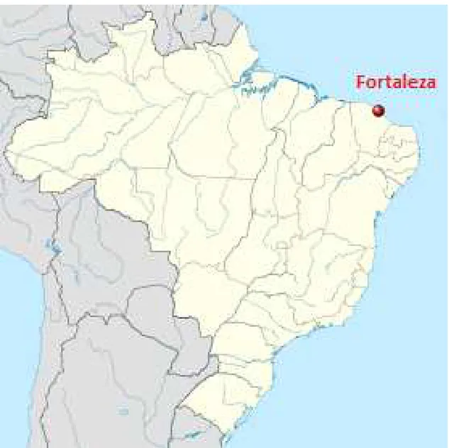
We have at our disposal information from a study field in the city of Fortaleza, Brazil (It is the state capital of Ceará, located in Northeastern Brazil. The city has a population close to 2.5 million and it is the 5th largest city in Brazil with an area of 313 square kilometers and one of the highest demographic densities in the country (8,001 perkm2_{), see the localization in Figure 1., page 6). The}

database houses information from a research project carried out by a group of researchers from UECE and UFC (State University of Ceara and Federal University of Ceara, respectively) for CAGECE (Water and Sewage Company of Ceara) (see, UECE, CAEN, and NPTEC (2006)). It applied more than 3,000 questionnaires containing socioeconomic and physical characteristics information from the household. Plus, CAGECE provided information about the monthly water consumption.

From a series of test procedures and econometric exercises, we confirm the importance of considering spatial effects, since the exclusion of those effects overestimates the impact of income and total of rooms over water demand while it underestimates the impact of average price and the total of residents. Although our results are of an exploratory nature, we believe they will open the way for a better understanding of how space matters for water micro demand estimation.

Besides this introduction and a section discussing final considerations, this paper has four more sections. Section 2 gives a brief explanation on how water is seen as an economic good, as well as a brief literature review on residential water micro demand estimation. Section 3 presents the database used in this work and the results of an exploratory spatial data analysis. Section 4 sets up the demand function to be estimated with a non-linear tax structure. Also, we present the econometric models used in this paper, such as the Spatial Error Model (SEM), the Spatial Autoregressive model (SAR) and the Spatial Autoregressive Moving Average model (SARMA), together with the tests used to (mis)specification analysis. Finally, Section 5 presents the results from the econometric model estima-tion.

2.

RESIDENTIAL WATER DEMAND

Over the last years, the perspective of water scarcity has become a pressing problem faced by humanity. The lack of such important natural resource produces a devastating effect on humanity. According to Europarl (2009), the spread of diseases by contaminated water represents 80% of the total of ill people and death in developing countries. Moreover, a lack of water to be used in agriculture could lead to absence of food, causing a scene of food insecurity in the planet (FAO, 2011). Among the causes that could lead the world into this dark picture of scarcity, we may quote the population growth, the changes in weather, the lack of good management practice of water resources and, overall, the pollution of water sources and the waste of it.

Figura 1: City of Fortaleza

maintenance of life in the planet. A report published by ISA (2007) (Socio Environmental Institute), estimated that in Brazil, in 2004, for every 100 liters of water taken from the sources that feed Brazilian capitals, 45 liters were lost in the distribution system. This value is extremely high if compared with countries like USA and France. In these countries the volume of wasted water reaches only 12 and 9 liters, respectively (Miranda and Koide, 2003).

But the waste of water does not occur in the distribution system only. It also occurs by the irrational and inefficient use by people in their households. While the per capita average consumption recommended by ONU is 110 liters of water per day, in Brazil the per capita average consumption is 150 liters per day, reaching 220 liters per day in capitals like Rio de Janeiro, Vitoria and Sao Paulo (ISA, 2007).

out the need to create policies that aims fighting against the potential lack of water in the planet. Until mid-1950, the policies to fight against a possible water scarcity focused in the supply side (Arbués, García-Valiñas, and Espiñeira, 2003). Such policies aimed the creation and enlargement of reservoirs, keeping the demand away from the main issue. From the beginning of the 1960s, and after the works of Gottlieb (1963) and Howe and Linaweaver (1967), it was realized that the best way to tackle water scarcity would be by controlling water demand. This process would avoid waste of water and would use it in a more effective way.

According to Milutinovic (2006) there are three ways to control water demand. The first one would be via price of water. The more people pay for water consumption the better they would use it in a rational way. The second way would be via public policies such as awareness of population, restrictions to water use etc. Finally, the last way would be by changes in technologies, developing new procedures that increase the efficiency of water use and decrease the consumption of it. In this work we will focus in control via price of water.

In the past, water did not have a price. It was regarded as a common good and it was avai-lable to the use of all. In classical economics, not only water but all the natural resources were regarded as determinants factors for production. In neoclassical economics, the natural resources were no longer seen as an obstacle to growth economic. For the neoclassical economists, the growing incorporation of technology in productive processes would solve the problem of natural resources scarcity so that economic growth would be continuous and not constrained. Besides that, they considered that natural resources were abundant and immutable, never facing scarcity. Therefore, natural resources were con-sidered common goods with no economic value and available for everyone to use it in the amount they wanted. So, natural resources, including water, were subject to the tragedy of common. This represents a situation in which a resource is overused (wasted) causing inefficiency and, consequently, a lack of the good.

From the mid-twenty century, when people realized the problem of scarcity, water began to be seen as an economic good and, thus it came to be valued. As Araújo (2007, p. 1) quoted, "the economic value of water is due to its scarcity". Therefore, the pricing of water is seen as a form of conservation and protection of such natural resource, as explained by the Dublin Statement (1992, apud ARAÚJO, 2007, p.1):

"Water has economic value in all of its uses and it must be recognized as an economic good ... . In the past, the not recognizing of water with economic value led to its waste and environmental damage resulting from its use. The management of water as an econo-mic good is an important way to reach efficiency and equity in its use, and to promote its conservation and protection".

To understand how charging water use affects its consumption, it is necessary to know the factors that determine water demand. As quoted by Gonçalves (2006) and Cohim, Garcia, and Kiperstok (2009), "the characterization of residential consumption is fundamental in determination of priority actions in the search for water rational use. In another words, the more detailed is the knowledge of consumption the more efficient is the demand management". In this sense, several studies have sought to characterize water consumption all around the world in order to provide a technical work that could be used as a support to implement policies aiming a more efficient water demand. Of course, for our purpose, the literature about econometric estimation of water micro demand embodies our way of characterizing the “structure” of water consumption under investigation. Next, we present a brief literature review on water demand estimation by econometric models.

3.

RECENT LITERATURE ON WATER MICRO DEMAND ESTIMATION

3.1 Traditional Models

Since the studies of Gottlieb (1963) and Howe and Linaweaver (1967), several researchers in many countries have carried out studies to estimate a residential water demand function for its regions in order to provide technical work as a support to implement policies aimed at controlling water demand and promoting its rational use and conservation.

Agthe, Billings, and Dobra (1986) in a study for Tucson, Arizona (USA) proposed a model where water demand was a function of marginal price, of difference, of family income, and of climate variable defined as evapotranspiration less precipitation in inches. To solve the problem of endogeneity, Agthe, Billings, and Dobra (1986) used an instrumental variable approach. The authors found that, except for family income, all the variables were statistically significant. Regarding the price elasticity of demand they found an estimated value of -0,624 indicating that water is a good with inelastic demand. Moreover, they found that water presents price elasticity of demand greater in the long run than in the short run, as most of commodities.

In a study carried out in Indonesia, Rietveld, Rowendal, and Zwart (1997) used Burtless and Hausman methods, by means of a maximum likelihood estimation. They used this technique to estimate a residential water demand function for the city of Salatiga in Indonesia. They used as independent variables: marginal price, number of residents, virtual income, a dummy that indicates if the residence has access to alternative source of water, and a variable defined as the output of virtual income and marginal price that aims to turn price elasticity into a changeable variable. Also, the authors showed that the only variable not statistically significant was the virtual income. Also, they found that the water demand in Salatiga is extremely sensitive to its price since the estimated mean value of price elasticity of water demand is -1.176, indicating that water demand in that region is elastic.

indirect way, by the income effect.

Finally, in Asia, Miyawaki, Omori, and Hibiki (2011) estimated the residential water demand in Japan. More specifically, in Tokyo and Chiba. They used as dependent variables: marginal price, vir-tual income, total of people living in the same house, total of rooms in the household, and the residence size. They used a maximum likelihood model. Miyawaki, Omori, and Hibiki (2011) pointed out that both the total of people living in the same house and the total of rooms presented a positive correlation with water demand. The residence size did not present any effect on water demand. As to the price elasticity of demand, the authors found an estimated value of -1.09, which means that in Japan water seems to be a good with elastic demand.

In Brazil, the literature about residential water demand estimation is still new. One of the first papers that had such approach was Andrade, Brandão, Lobão, and Silva (1995). They estimated a function of residential water demand for the state of Parana. In order to determine which factors affect water demand, the authors used the following variables: marginal price, difference, income and total of people living in the househould. Since Sanepar (Sanitation Company of Parana) adopted a tax structure in rising block, the authors faced a problem with endogeneity. To solve this problem they used McFadden method. This method creates a proxy variable to marginal price, not correlated to random error. Andrade, Brandão, Lobão, and Silva (1995) found that the marginal price elasticity of demand is inelastic. The estimated price elasticity is -0.24 indicating that a reduction in water consumption occurs in a lower proportion than a price increasing. As to the difference elasticity, the authors found an estimated elasticity of 0.05. The positive value indicates an embedded subsidy for families who consumed from 10m3_{and up. In other words, for those families who consumed from the second block}

of consumption and on. Regarding the income and the total of people in the same house, the authors found that income does not have a significant effect on water consumption. The explanation for such result would be the lack of variability in family size presented in the sample.

Estimating a residential water demand for the city of Piracicaba, São Paulo, Mattos (1998) proposed that the variables determining residential water demand in that city would be the marginal price, difference, total of residents, familiar income, temperature and precipitation. Mattos (1998) used the OLS model, the instrumental variable, the McFadden method and the 2SLS model. Mattos (1998) found that only the marginal price and the difference were significant, explaining 71% of water con-sumption variation. They found an estimated value of -0.21 for the price elasticity of demand. This value is very close to the one found by Andrade, Brandão, Lobão, and Silva (1995).

Using data from “Banco do Nordeste” (BNB), Melo and Neto (2007) estimated a function of residential water demand for Northeast of Brazil. The variables explaining water demand were be average price, marginal price, income, how long the residents were living in the same place, total of room, and the average age of the head of household. To solve the problem of endogeneity due the rising blocks tax, Melo and Neto (2007) used Burtless and Hausman method. Such methods aggregate the information about the entire consumer’s budget constraints, modify the problem of maximization, turn the budget constraints into non linear function, and remove the bias caused by traditional methods (Melo and Neto, 2007).

price, difference, family income, total of people living in the same residence, total of rooms, monthly average temperature, assessment from consumer about the quality of consumed water, assessment from consumer about the regularity of water supply, plus an assessment from consumer regarding quantity of consumed water. To solve the problem with endogeneity, Brasil (2009) estimated the pro-posed model via clustered OLS using first differences. She showed that an increase of $1 real in both average price and difference is responsible for a decrease of water consumption of 0.56m3 _{and 0.23}

m3_{, respectively.}

3.2 Models that Incorporate Spatial Effects

When we handle data that deals with location, it comes out two types of problem that, if ig-nored, it may cause serious problems to the estimative obtained by traditional econometric techniques. Such problems are: spatial dependence and spatial heterogeneity. For spatial dependence we mean a situation where an observation of a given variable at placeidepends on the observations in other locationj6=i. According to LeSage (1999), there are two reasons why such spatial dependence exists in a sample. The first one would be measurement error. In a sample created from observations as-sociated to spatial units, such as municipalities, states, census divisions and so on, the administrative boundaries may not reflect, in an accurate way, the nature of the process that is being analyzed. Now, according to Anselin (1988), the second factor that causes spatial dependence in a sample "is the most fundamental and comes from the importance of space as an element in the construction of explanation on human behaviour". Still according to him, "the essence of regional science and human geography is that both location and distance are important, and the result is variety of interdependence in space and time". Thus, it is expected that there is spatial dependence in situations where both sociodemo-graphic and economic characteristics, plus the regional activity, are an important aspect for modeling the problem.

Spatial heterogeneity refers to a situation where the relation among variables varies in space. In other words, there is a different relation in each point of space (LeSage, 1999). Anselin (1988) says that besides this lack of stability in relations through space, the region heterogeneity -that in general has different socioeconomic characteristics - is measured by error, what may cause heterocedasticity.

Thereby, we need a new theoretical approach to model problems where spatial issue has an important role to explain the phenomenon studied. In this sense, spatial econometrics has been used to explain several socioeconomic problems - such as problems related to regional development, criminality, contagion and, of course, residential water demand. However, in the specific case of water demand there are few studies in international literature and none in the national one.

association patterns, which is the spatial correlation of errors.

Aware over this problem, some authors started to include spatial effect in their analysis and sought to explain the spatial association pattern for water consumption. Wentz and Gober (2007) used GWR model (Geographic Weighted Regression) in a study for Phoenix, USA to verify if there was any additional contribution of spatial effect over the results obtained by OLS model (Ordinary Least Square). The authors verified, by means of the GWR model, that the importance of spatial effects reduces to two variables that determine water demand. The variables are: residence size and if there was a swimming pool in the residence. In another words, since there is a spatial pattern of residential distribution that has those characteristics, these variables represent similar water consumption. They found that any policy that aims decreasing water consumption by controlling the construction of swimming pools, the residence land size, or the type of vegetation in garden’s house, will have different effects on different parts of the city. This conclusion was possible due to the fact that GWR model estimates a different coefficient for each region in the city.

For the state of Oregon (USA), Franczyk and Chang (2008) realized that water demand was not explained by both population and economic growth only, but also by other biophysical and socioeconomic factors that in general present spatial dependence. The authors used Spatial Erros Model (SEM), besides the OLS model, to include spatial autocorrelation effects into the problem. They used Moran-I statistics and showed that there is spatial dependence of errors. Also, they found that the inclusion of such effect increases the significance of factors that determine water demand.

For the city of Portland (Oregon, USA) Chang, Parandvash, and Shandas (2010) identified a spatial association pattern for water demand. They identified that the areas where water consumption was higher coincided with the areas which the residence size was big and with the areas where both building density and age of buildings were low. Besides the OLS and SEM models, the authors used the Piecewise Linear Regression model (PWLR), dividing both the residence size and the building density into two ranges. As in the Franczyk and Chang (2008)’s work, the model that better explained water consumption variability was the SEM model.

House-Peters, Pratt, and Chang (2010), in a study for the city of Hillsboro (Oregon, USA), analyzed the climate effects on water demand. Using spatial analysis techniques, the authors found that, although water demand in that area was not sensitive to dry conditions at all, specific areas presented higher water consumption under such conditions. Also, the authors showed that in areas where water demand is more sensitive to weather, these areas presented higher concentration of new and big residences, with high value and with residents with higher education level.

In Brazil, the literature about spatial effects on water demand econometric estimation does not exist. In this sense, this work aims to fill this gap aggregating such effects in the analysis of residential water demand in Fortaleza. Next section will present the database used in this work. Also, it will be carried out an exploratory analysis over the data.

4.

DATA SET

4.1 The Sample

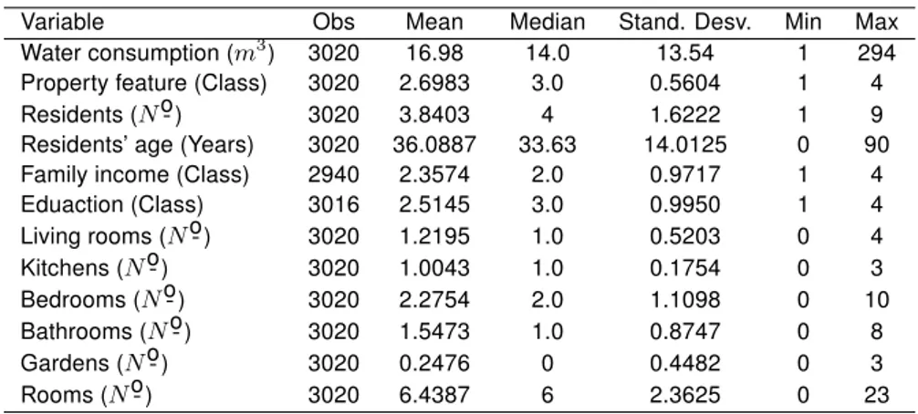
A total, 5,444 interviews were conducted in 56 municipalities of Ceara in February, 2007. Also, CAGECE tracked water consumption during 10 months (from August, 2006 to May, 2007) in the residences that participated in the survey (Brasil, 2009). Since our main goal was to estimate residential the water demand for the city of Fortaleza, we collected only information over consumers from that city. Thus, the final sample for the city of Fortaleza has 3,020 observations, as shown in Table 1.

Tabela 1: Descriptive Statistics of Variables

Variable Obs Mean Median Stand. Desv. Min Max Water consumption (m3_{) 3020 16.98 14.0 13.54 1 294}

Property feature (Class) 3020 2.6983 3.0 0.5604 1 4 Residents (No_{¯ )} 3020 3.8403 4 1.6222 1 9 Residents’ age (Years) 3020 36.0887 33.63 14.0125 0 90 Family income (Class) 2940 2.3574 2.0 0.9717 1 4 Eduaction (Class) 3016 2.5145 3.0 0.9950 1 4 Living rooms (No_{¯ )} 3020 1.2195 1.0 0.5203 0 4 Kitchens (No_{¯ )} 3020 1.0043 1.0 0.1754 0 3 Bedrooms (No_{¯ ) 3020 2.2754 2.0 1.1098 0 10} Bathrooms (No_{¯ )} 3020 1.5473 1.0 0.8747 0 8 Gardens (No_{¯ ) 3020 0.2476 0 0.4482 0 3} Rooms (No_{¯ )} 3020 6.4387 6 2.3625 0 23 Source: Elaborated by authors

The data presented shows that residential water consumption in February 2007 for the city of Fortaleza was 16.98 m3_{, on average. The median of 14 m}3 _{indicates that half of residences in}

Fortaleza are in CAGECE’s second consumption block2_{(10 m}3 _{to 15}

m3_{). This might be not good for}

CAGECE if the tax structure is poorly designed.

As to socioeconomic characteristics, on average, each household has 4 residents and these residents are 36 years old. The families have an average monthly income of 2.35, which indi-cates that these families are between the class that earns more than a minimum wage and up to 2 minimum wage, and the class that earns 2 minimum wage and up to 5 minimum wage. For educa-tion, the respondents’ average education was 2.51, something between the class that has fundamental education and the class that has completed high school.

As to the physical characteristics of households, the residences have, on average, 6.5 ro-oms, distributed in the following (on average): 1.21 living roro-oms, 1 kitchen, 2.27 bedroro-oms, 1.54 bath-rooms and 0.24 gardens. The average rating of property feature is 2.69, indicating that the residences are classified between medium and regular categories.

Turning into the issue of prices, CAGECE applies an increasing tariff system in consump-tion blocks, as shown in Table 2. The tariff structure applied by the company looks for the following: i) allow all citizens access to services; ii) encourage rational water use; iii) finance the continued deli-very of services; iv) allow investments to expand services; and v) maintain the economic and financial stability.

Tabela 2: Values of Tariff Structure by Consumption Group - February, 2007

Water consumption (m3) Price bym3

[0 , 10] R$ 0.98

(10 , 15] R$ 1.56

(15 , 20] R$ 1.65

(20 , 50] R$ 2.80

(50 ,∞) R$ 4.95

Source: Elaborated by authors

In this charging mechanism, the price paid by consumer is calculated in a “cascade way”; in another words, the total amount consumed is divided into consumption blocks where each part is charged by the rate established to that block as shown in the Equation 1.

P =

                  

0,98.10,ifq∈[0,10]

0,98.10 + 1,56.(q−10),ifq∈(10,15]

0,98.10 + 1,56.5 + 1,65.(q−15),ifq∈(15,20]

0,98.10 + 1,56.5 + 1,65.5 + 2,80.(q−20),ifq∈(20,50]

0,98.10 + 1,56.5 + 1,65.5 + 2,80.30 + 4,95.(q−50),ifq∈(51,∞)

(1)

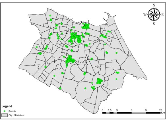
Finally, since our focus is the spatial effect on water demand, Figure 2 presents the sam-ple’s spatial distribution over the city of Fortaleza. We can see a relatively well distributed pattern. However, some neighborhoods (bairros) are highlighted, such as: Centro, Praia de Iracema, Benfica, bairro de Fátima, Itaperi, Serrinha and Messejana.

There are two possible criticisms that may arise regarding the use of this database: the first one is that the sample was not developed for the city of Fortaleza; the second one is the presence of clusters. To justify the first problem, due to technical impossibility to georeference all address in inner cities of Ceara, we preferred to use data for the city of Fortaleza only. Regarding the presence of clusters in the sample, we are aware that this problem may affect the coefficient estimatives. However, we will ignore such possibility, since we do not have a specific sample set up for a spatial analysis. Now that the database and its spatial distribution were presented, an exploratory analysis over the data will follow.

4.2 Spatial Exploratory Data Analysis

Figura 2: Sample Spatial Distribution byBairros ! ( ! (!(!(!(!(!(!( ! ( ! ( ! ( ! ( ! ( ! ( ! (!(!( ! (((!(!(!(!(!(!!!!((!(!(!(!(((!!(!(!(!(!(!!(!(!( ! ( ! ( ! (!(!( ! (!(!(!( ! ( ! ( ! ( ! ( ! ( ! ( ! (!(!( ! ( ! ( ! (!!((!(!(!(!(!((!!(!(!(!(!(!(!(((!!!(!(!(!(!(!(!(!!((!(!(!(!(!(!( ! ( ! ( ! (!(!( ! ( ! ( ! (!( ! ( ! ( ! ( ! ( ! ( ! ( ! ( ! ( ! ( ! ( ! ( ! ( ! ( ! ( ! ( ! ( ! ( ! ( ! ( ! ( ! (!(!(!(!(!( ! ( ! ( ! ( ! ( ! ( ! ( ! ( ! ( ! (_{(!(!(!(!!(!(!(!!(!(!((}(!(!(!!(!(!((!!!(!(!((((!(!(!!!(!(!(!!!(((!(!(!((!(!!(((!(!(!(!(!(!(!((!(!(!(!!((!((!!(!!(!(!(!(!(!(!(!(!(!(!(!(!(!!!!((!(!(!(!(!(!(((!(!!(!(!!(!!(!(!(!(!((((!!!(!(!(!(!(!(!(!!_(!(!(!(!(!(_!(!(!(!(!(_(!!!!(!(((!(((!(!(!(!(!(!(!!!(!((((!!(!(₍!!(!(!!_!(!((!(!((!!(!(!(!!!(!(!(!(!(!((!(((!!(!(!(!(!((!(!(!(!(((!(!((!!!!((!(!(!(!!((!(!(!((!!(!(!!(!(_!((!(!!(!(!!(!((!(!!(!(!(!(!(!(((!!(!((!!(!!!(!(!(!((!((!!(!(!( ! ( ! ( ! (!(!(!( ! ( ! ( ! ( ! ( ! ( ! ( ! ( ! ( ! ( ! ( ! ( ! ( _!(!( ! ( ! ( ! ( ! ( ! (!( ! ( ! ( ! ( ! ( ! ( ! ( ! ( ! ( ! ( ! ( ! ( ! ( ! ( ! ( ! ( ! ( ! ( ! ( ! ( ! ( ! ( ! ( ! ( ! ( ! ( ! ( ! ( ! ( ! ( ! ( ! ( ! ( ! ( ! ( ! ( ! ( ! ( ! ( ! ( ! ( ! ( ! ( ! ( ! ( ! ( ! ( ! ( ! ( ! ( ! ( ! ( ! ( ! ( ! ( ! ( ! ( ! (!( ! ( ! ( ! (_!( ! ( ! ( ! ( ! ( ! ( ! ( ! (!(!(!!(!(!(!(!((!(!(!((!!(!((!(!(!!( ! ( ! (!( ! ( ! ( ! ( ! ( ! ( ! (!(!( ! ( ! ( ! ( ! ( ! ( ! ((!(!(!!(!(!(!((!!(_!((((!!!(!(!(!(!(!(_(!!!(!((!!!((!((!(!(!!(!((_(!(!! ! (!(!(!( ! (!(!(!(!((!((!!(!!!((!(!(!(!(!!(!((!((!(!(!(!!(!(!(!(!(!(!(_!( ! ( ! ( ! ( ! ( ! ( ! ( ! ( ! ( ! ( ! ( ! ( ! ( ! ( ! ( ! (!( ! ( ! ( ! (!(!(!( ! ( ! ( ! ( ! ( ! ( ! (!(!( ! (!(!(!(!(!( ! ( ! ( ! ( ! (!( ! ( ! ( ! ( ! ( ! (!((!!!(!(!((((!!(!(!(!(!!((!(((!!!(!!(_!(!(!(!(!!(!(!!(((!(((!(!(!(!!((!(!!(!!(!(!( ! (!!(!(!(!(!(!(!((((!(!(!(!(!(!!(!(!!(!(!(!(!!(( ! ( ! ( ! ( ! ( ! ( ! ( ! ( ! ( ! ( ! ( ! (!(!( ! ( ! ( ! ( ! (((!(!(!(!(!(!!!(!(!(!(!(!(!!((((!(!(!(!(!!(((!((!!!(!((!(!(!(!(!!!!(!(!!((!(!(!(!(!(((!!(!(!(((!(!!(!!!(!!(!(((!(!!!(!(!(!!(!(!((!!(!((!(( ! (!(!( ! ( ! (!(!( ! ( ! ( ! ( ! ( ! ( ! (!(!( ! ( ! ( ! ( ! ( ! ( ! ( ! ( ! ( ! ( ! ( ! ( ! ( ! ( ! ( ! ( ! ( ! ( ! (!(!( ! ( ! (!(!(!(!( ! ( ! ( ! ( ! ( ! ( ! ( ! ( ! ( ! ( ! ( ! (((!!!(!(!(!(!(!(!(!( ! (!(!( ! ( ! ( ! (!(!(!( ! ( ! ( ! ( ! ( ! ( ! (!(!(!(!(!( ! ( ! ( ! ( ! ( ! (_!(!(!(_!( ! ( ! ( ! ( ! ( ! ( ! ( ! ( ! ( ! ( ! (!(!(!(!(!(!(!( ! (!(!( ! ( ! ( ! (!( ! ( ! ( ! ( ! ( ! (!( ! ( ! (!( ! ( ! ( ! ( ! ( ! ( ! ( ! ( ! (!!(!((!(!((!(!(!(!!!!(!(!((!((((!(!(!(!(!!!(!(!(!(!((!(!(!(!!(!(!(!( ! ( ! ( ! ( ! ( ! ( ! ( ! ( ! ( ! ( ! ( ! ( ! (!(!(!(!(!(!( ! ( ! (!!(((((!(!(!!!(!(!(!(! ! (!(!( ! ( ! (!(!(!( ! (!( ! ( ! ( ! ( ! ( ! ( ! (!(!( ! ( ! ( ! ( ! ( ! ( ! (!(!( ! ( ! ( ! (!( ! ( ! ( ! ( ! ( ! ( ! ( ! ( ! ( ! ( ! ( ! ( ! ( ! ( ! ( ! ( ! ( ! ( ! ( ! ( ! ( ! ( ! ( ! ( ! ( ! (!(!(!(!(!(!((!!(!(!(!(!(!!((((!(!!!(!!(((!(!(!(!(!!(!((!(! ! ( ! ( ! ( ! ( ! ( ! ( ! (!(!(_!( ! ( ! ( ! ( ! ( ! (!( ! ( ! ( ! ( ! ( ! ( ! ( ! ( ! ( ! ( ! ( ! (!( ! ( ! ( ! ( ! ( ! (!(!((!(!(!(!!((!(!!(!(!(!!(!((!(!(!!((!(!(!!(!(!((!(!(((!(!!((!!!(!((!!!(!((!(!(!!((!(!(((!!!(!(!((!!(!(!((!!(_!( ! ( ! ( ! ( ! ( ! ( ! ( ! ( ! ( ! ( ! ( ! ( ! ( ! (!(!(!(!(!!(!((!(((!!!(!(!(!!(!((!(!((! ! ( ! ( ! ( ! ( ! ((!(!(!(!!(!(!(!(!( ! ( ! ( ! ( ! ( ! ( ! ( ! ( ! ( ! ( ! ( ! ( ! ( ! ( ! ( ! (!(!(!( ! (!( ! (!(!( ! ( ! (!(!(!((!!(!(!(!( ! ( ! ( ! ( ! ( ! ( ! ( ! ( ! ( ! ( ! ( ! ( ! ( ! ( ! ( ! ( ! ( ! ( ! ( ! ( ! ( ! ( ! ( ! ( ! ( ! ( ! ( ! ( ! (!( ! ( ! ( ! ( ! ( ! ( ! ( ! ( ! ((!(!(! !!(!(!(!(!(!((!((!(!(!!!(( !(!(!( ! ( ! ( ! ( ! ( ! ( ! ( ! (!!(!(!((!!(((!(! ! ( ! ( ! ( ! ( ! ( ! ( ! ( ! ( ! ( ! (!(!(!(!(!(!(!( ! ( ! ( ! ( ! ( ! ( ! ( ! ( ! (!(!(!(!( ! ( ! ( ! ( ! ( ! ( ! ( ! ( ! ( ! ( ! ( ! ( ! ( ! ( ! ( ! ( ! ( !(!( ! ( !(!( ! ( _!(!( ! ( ! ( ! ( ! ( ! ( ! ( ! ( ! ( ! ( !( !( ! ( ! ( ! (!(!( ! ( !(!( ! ( ! ( !(!(!( ! ( ! ( ! ( ! ( ! ( ! ( ! ( ! ( ! ( ! ( ! ( ! ( ! ( ! ( !!(!(!(!(!(!!!(((!(!(!(!(!(!(!((!(!(!((! ! ( ! ( ! ( ! ( ! ( ! ( ! (!(!( ! ( ! ( ! ( ! ( ! ( ! ( ! ( ! ( ! (!( ! ( ! ( ! ( ! ( ! ( ! ( ! ( ! ( ! ( ! ( ! (!( ! ( ! ( ! ( ! ( ! ( ! ( ! ( ! ( !( ! ( ! ( ! ( ! ( ! ( ! ( ! ( ! ( ! ( ! (!( ! ( ! ( ! ( ! ( ! ( ! ( ! (!(!(!( ! (_!( ! ( ! ( ! ( !( ! ( ! ( ! (!( ! ( ! ( ! ( ! ( ! ( ! ( ! ( ! ( ! ( ! ( ! ( ! ( ! ( ! ( ! ( ! ( ! ( ! ( ! (!( ! ( ! ( ! ( ! ( ! ( ! ( ! ( ! ( ! ( ! ( ! (!( ! ( ! ( ! ( ! ( ! ( ! ( ! ( ! ( ! (!( ! ( ! ( ! ( ! ( ! ( ! ( ! ( ! ( ! ( ! ( ! ( ! ( ! ( ! ( ! ( ! ( ! ( ! ( ! ( ! ( ! ( ! ( ! ( ! ( ! ( ! ( ! ( ! (!( ! ( ! ( ! (_!( ! ( ! ( ! ( ! ( ! ( ! ( ! ( ! ( ! ( ! ( _!( ! ( ! ( ! ( ! ( ! ( ! ( ! ( ! ( ! ( ! (!(!(!(!(!( ! ( ! ( ! ( ! ( ! ( ! ( ! ( ! ( ! ( ! ( ! ( ! ( ! ( ! ( ! ( ! (!( ! ( ! ( ! ( ! ( ! ( ! ( ! ( ! ( ! (!(!( ! ( ! ( ! ( ! ( ! ( ! ( ! ( ! ( ! ( ! ( ! ( ! (!(!(!(!(!(!(!(!((!!(((!!!(!(!( ! (_!( ! (!(!( ! ( ! ( ! ( ! ( ! (!((!_{!(!(!(!(((!(!(!(!(!!(!!(}(!(!!(!(!(!(!!(!(( ! ( ! (!(!(!((!!(!(!(_!( ! ( ! ( ! ( ! ( ! ( ! ( ! ( ! ( ! ( ! ((!!(!((!(!(!!(!( ! ( ! ( ! ( ! ( ! ( ! ( ! ( ! ( ! (!!(!(!((!!(!(!(( ! ( ! ( ! ( ! ( ! ( ! (!(!(!(!(!(((!!(!(!(!(!!(!(!(!(!((!(!!(!(!(!(!(!((!(!!(!(!(!!!((!((!((!(((!(!(!!! ! ( ! ( ! ( ! ( ! ( ! ( ! ( ! (_(!(!!((!(!_{!(((!(!(!(!!!(!((!(!} ! ( ! ( ! ( ! ( ! ( ! ( ! ( ! ( ! ((!(!(!!(!(!(!((!(!(((!!!(!(!(!(!(!((!(!(!(!(!(!(!!!((!(!(!(!(!!(!(!(!(!(!( ! ( ! (_!( ! ( ! ( ! ( ! ( ! ( ! ( ! (!(!(!(!((!(!(!!!(!(!(!(!(((!(!(!!(!(!(!( ! ( ! ( ! ( ! ( ! ( ! ( ! ((!(!(!(!(!(!(!!!(!(!(!(!(!(!(( ! ( ! ( ! ( ! ( ! ( ! ( ! ( ! ( ! (!(!(!(!!!(!((((!(!(!(!(!(!!(!(!(!(!(!((! ! ( ! ( ! ( ! ( ! ( ! (!(!( ! (!( ! ( ! ( ! ( ! ( ! ( ! ( ! ( ! ( ! ( ! ( ! ( ! ( ! (!(!(!(!(!(!( ! ( ! ( ! ( ! ( ! ( ! ( ! ( ! ( ! ( ! (!( ! ( ! ( ! ( ! ( ! ( ! ( ! ( ! ( ! ( ! ( ! ( ! ( ! ( ! ( ! ( ! ( ! ( ! ( ! (!(!( ! ( ! ( ! ( ! ( ! ( ! ( ! ( ! ( ! ( ! ( ! ( ! ( ! ( ! (!(!(!(!( ! (!(!(!!((!(!(!(!(!(!( ! ( ! ( ! ( ! ( ! ( ! ( ! ( ! ( ! ( ! ( ! ( ! ( ! (!(!(!!(!(!(!(!(((!!!!(((!(!(((!(!(!(!(!!!!(!((((((!(!!!(!(!!(!(!(!(!(!!(!(!(!((!(!((!(!(!(!!!(((!((!(!!!!!(((!(!(!(!(!(!(!(!!(!((!(!_!((!(!(! ! ( ! ( ! ( ! ( ! ( ! ( ! ( ! ( ! (!(!(!(!(!( ! ( ! ( ! ( ! ( ! ( ! ( ! ((!(!(!(!((!!!(!((!!!(!((!(!(!( ! ( ! ( ! ( ! ( ! ( ! ( ! ( ! ( ! ( ! ( ! ( ! ( ! ( ! ( ! ( ! ( ! ( ! ( ! (!(!(!( ! ( ! ( ! ( ! ( ! ( ! (!(!( ! ( ! ( ! ( ! (!(!(!(!(_!( ! ( ! ( ! ( ! ( ! (!!(!(!(!(!((!!(!(!(!(!(( ! ( ! ( ! ( ! ( ! ( ! ( ! ( ! ( ! (!( ! ( ! ( ! (!!((!(!!!(!((!(( ! ( ! ( ! (!(!(_!(!(!( ! ( ! ( ! ( ! ( ! ( ! ( !₍(!(!(_!!!((!(!(!( ! (!!(!((!!((_!(!(!( ! ( ! ( ! ( ! ( ! ( ! (!(!( ! ( ! ( ! ( ! ( ! ( ! ( ! ( ! ( ! ( ! (!((!!(!((!(!(!(!(!!(!(!(!(!(!( ! ( ! (!( ! ( ! ( ! ( ! ( ! ( ! ( ! ( ! ( ! ( ! ( ! ( ! ( ! ( ! ( ! ( ! ( ! ( ! ( ! ( ! ( ! ( ! ( ! ( ! ( ! ( ! ( ! ( ! ( ! ( ! ( ! ( ! ( ! ( ! ( ! ( ! ( ! ( ! ( ! ( ! ( ! ( ! ( ! ( ! (!!(!!((((!(!!(!(!(((!!(!(!(!(!(!(!!( ! ( ! ( ! ( ! ( ! ( ! ( ! ( ! ( ! ( ! ( ! ( ! ( ! ( ! ( ! ( ! ( ! ( ! ( ! ( ! ( ! ( ! (!( ! (!(!(!(!(!(!(!( ! ( ! ( !( ! (!(!( ! ( ! ( ! ( ! ( ! ( ! ( ! ( ! ( ! ( ! ( ! (!(!(!( ! ( ! ( ! ( ! ( ! (!(!(!(!( ! (!(!(!( ! ( ! ( ! ( ! ( ! ( ! ( ! ( ! ( ! ( ! ( ! ( ! ( ! ( ! ( ! ( ! (!(!(!(!(!(!( ! (!(!(!( ! ( ! ( ! ( ! ( ! ( ! ( ! ( ! (!( ! (!(!(!( ! (!( ! ( ! ( ! ( ! ( ! ( ! ( ! ( ! ( ! ( ! ( ! ( ! ( ! ( ! ( ! ( ! ( ! ( ! ( ! ( ! ( ! ( ! ( ! ( ! ( ! ( ! ( ! (!( ! ( ! ( ! ( ! ( ! ( ! ( ! ( ! ( ! ( ! ( ! ( ! (!( ! ( ! ( ! ( ! ( ! (!(!(!(!(!(!( ! ( ! ( ! ( ! ( ! ( ! ( ! (!!(!(!((!((!(!(!(! ! ( ! ( ! ( ! ( ! ( ! ( ! ( ! ((!(!(!(!(!!!(!(((!(!!!(!(!(!((!(!(!((! ! ( ! (!(!(!( ! ( ! ( ! ( ! ( ! ( ! ( ! ( ! (!(_!(!(!( ! ( !( ! ( ! ( ! ( ! ( ! ( ! ( ! ( ! ( ! ( ! (!( ! ( ! ( ! ( ! ( !( ! ( ! ( ! ( ! (!(!( ! ( ! ( ! ( ! ( ! ( ! ( ! ( ! ( ! ( ! ( ! ( ! ( ! ( ! ( ! ( ! ( ! ( ! ( ! ( ! (!( ! ( ! ( ! ( ! ( ! ( ! ( ! ( ! ( ! ( ! ( ! ( ! ( ! (!( ! (!(!(!(!( ! ( ! ( !( ! ( ! ( ! ( ! ( ! (!( ! ( ! ( ! ( ! ( ! ( ! ( ! ( ! ( ! ( ! ( ! ( ! ( ! ( ! ( ! ( ! ( ! ( ! ( ! ( ! ( ! ( ! ( ! ( ! ( ! ( ! ( ! ( ! ( ! ( ! ( ! ( ! (!( ! ( ! ( ! ( ! ( ! ( ! (!(!( ! ( !( ! ( ! ( ! ( ! ( ! ( ! ( ! ( ! ( ! ( ! ( ! (_!( ! ( ! ( ! ( ! ( ! ( ! ( ! ( ! ( ! ( ! ( ! ( ! ( ! ( ! ( ! ( ! ( ! ( ! ( ! (!( ! ( ! ( ! ( ! ( ! ( ! ( ! (!(!( !( ! ( ! ( ! ( ! ( ! (!(_!(!(!(!( ! ( ! ( ! ( ! ( ! ( ! ( ! ( ! ( ! ( ! ( ! (!( ! ( ! ( ! ( ! ( ! ( ! ( ! ( ! ( ! ( ! ( ! ( ! ( ! ( ! ( ! ( ! ( ! ( ! ( ! ( ! ( ! (!( ! (_!( ! ( ! ( ! ( ! ( ! ( ! ( ! ( ! ( ! ( ! (!( ! ( ! ( ! ( ! ( ! ( ! ( ! ( ! ( ! ( ! ( ! ( ! ( ! ( ! ( ! ( ! ( ! ( ! ( ! ( ! ( ! ( ! ( ! ( ! ( ! ( ! ( ! ( ! ( ! ( ! ( ! ( ! ( ! ( ! ( ! ( ! ( ! ( ! (!(!( ! ( ! ( !( ! ( ! ( ! ( ! ( ! ( ! ( ! ( ! ( ! ( ! ( ! ( ! ( ! ( ! ( ! ( ! ( ! ( ! ( ! ( ! ( ! ( ! ( ! ( ! ( ! ( ! ( ! ( ! ( ! ( ! ( ! ( ! ( ! ( ! ( ! ( ! ( ! ( ! ( ! ( ! ( ! ( ! ( ! ( ! ( ! ( ! ( ! ( ! ( ! ( ! ( ! ( ! ( ! ( ! ( ! (!( ! ( !( ! ( ! ( ! ( ! ( ! ( ! ( ! ( ! ( ! ( ! ( ! ( ! ( ! ( ! ( !( ! ( ! ( ! ( ! ( ! ( ! ( ! ( ! ( ! ( ! ( ! ( ! ( !( ! ( ! (!( ! ( ! ( ! ( !(!( ! ( ! ( ! ( ! ( ! ( ! ( ! ( ! ( ! ( ! ( ! ( ! ( ! ( ! ( ! ( ! ( ! ( ! ( ! ( ! ( ! ( ! ( ! ( ! ( ! ( ! ( ! ( ! (!(!(!( ! ( ! (!( ! ( ! ( ! ( ! ( ! ( ! ( ! ( ! ( ! ( ! ( ! ( ! ( ! ( ! ( ! ( ! ( ! ( ! ( ! ( ! ( ! ( ! ( ! ( ! ( ! ( ! ( ! ( ! ( ! ( ! ( ! ( ! ( ! ( ! ( ! ( ! ( ! (!( ! ( ! ( ! ( ! ( ! ( ! ( ! ( ! ( ! ( ! ( ! ( ! ( ! ( ! ( ! (!( ! ( ! ( ! ( ! ( ! ( ! ( ! ( ! ( ! ( ! ( ! ( ! ( ! ( ! (!( ! ( ! ( ! ( ! ( ! ( ! ( ! ( ! ( ! ( ! ( ! ( ! ( ! ( ! ( ! ( ! ( ! ( ! ( ! ( ! ( ! ( ! ( ! ( ! ( ! ( ! ( ! ( ! ( ! ( ! ( ! ( ! ( ! ( ! ( ! ( ! (!( ! ( ! ( ! ( !( ! ( ! ( ! ( ! (!( ! (!( ! ( ! ( ! ( ! ( ! (

0 1,5 3 6 9 12

Km

µ

Legend

!

( Sample City of Fortaleza

Tabela 3: Moran-I Statistic for Water Consumption

Moran-I statistic Mean Variance p-value 0,039365 -3.31e-04 6.0e-07 <2.2e-16 Source: Elaborated by authors

Nota: empirical p-value based on randomization method

The results presented in Table 3 show that Moran-I is 0.03, a value that exceeds the statis-tical average, but it is very close to zero, which indicates that there is no spatial autocorrelation in water consumption. However, although this value is close to zero, it is statistically different from zero, once the pseudo p-value is extremely low and indicates that there is a positive spatial autocorrelation, even in a very reduced magnitude.

However, not always the global pattern of spatial association reflects the local pattern of spatial association. Anselin (1995) asserts that global statistics of spatial association are not able to identify the occurrence of local autocorrelation, since the global statistics may hide local association patterns through indication of global autocorrelation absence, or may mask the association patterns as clusters or spatial outliers through indication of a strong global autocorrelation. In this sense, the LISA index (Local Indicator Spatial Association) is used to overcome this obstacle and capture local patterns of linear association.

Ii = (yi−y)

P

jwij(yj−y)

P

i(yi−y)2/n

(2)

Where:

n= number of observations

yi = observation for the studied variable in regioni yj = observation for the studied variable in regionj y= mean for the studied variable

wij = matrix element W that corresponds to distance betweeniandjregions.

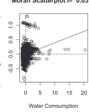
According to Almeida (2004), "the intuitive interpretation is that the local Moran-I provides an indication of the clustering degree of similar values around a specific observation, identifying spatial clusters statistically significant". In order to analyze the local Moran-I, we used the Moran dispersion diagram and both the Moran dispersion (clusters) and the significance maps, which are presented next. The diagram is a way to interpret the Moran-I statistic. The Moran-I is the angular coefficient of a regression between the variable under analysis and its spatially lagged values3_.

Figura 3: Moran Dispersion Diagram

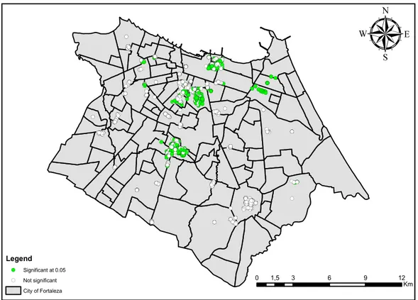
The results presented in the dispersion diagram (see, Figure 3) show that there is a ten-dency of positive autocorrelation with the observations distributed in the first and third quadrants. As to the significance map, Figure 4(a), on page 17, shows some clusters that are not significant, being represented in white, while the significant clusters are presented in green.

4(b), on page 17) show that there is a high concentration of water consumption at the top center in the city of Fortaleza, represented by the red dots that covers downtown area and the richest neigh-borhoods in capital. However there are low consumption clusters that are represented by blue dots in suburbs areas. Although almost imperceptible, there is a set up of low-high clusters at the top center, where is located the high-high cluster indicating that there are residences that have low water consump-tion, although these residences are located in rich areas. Also there is a set up of high-low clusters in suburbs, where there are residences that have high consumption in region where there is low consump-tion. A possible explanation for the configuration of such clusters is that the income distribution in the city of Fortaleza is unequal. In some popular neighborhoods there are some residents with a very high income level comparing to those who live in the same area. The same pattern takes place in the rich areas, where there are very poor residents living in such rich neighborhoods.

Figura 4: Significance and Dispersion Maps ! ( ! (!(!(!(!(!(!( ! ( ! ( ! ( ! ( ! ( ! ( ! (!(!( ! (!(!(!(!(!(!!!(!((((!(!!!((!((!(!!(!(!(!(!(!(!( ! ( ! ( ! (!(!( ! (!(!(!( ! ( ! ( ! ( ! ( ! ( ! ( ! (!(!( ! ( ! ( ! (!(!(!(!(!(!(((!!!((!(!!(!!((((!(!(!!!!(!(!(!(!(!(!(!((!((!(!(!(! ! ( ! ( ! ( ! ( ! ( ! ( ! ( ! (!( ! ( ! ( ! ( ! ( ! ( ! ( ! ( ! ( ! ( ! ( ! ( ! ( ! ( ! ( ! ( ! (((!!!(!(!(!(!(!(!(!( ! ( ! ( ! ( ! ( ! ( ! ( ! ( ! ( ! (_{(!(!(!(!!(!(!(!!(!(!((}(!(!(!!(!(!(!((!(!(!(!(((!(!!(!(!(!!(((!(!(!!!(!(!!(!(!(((!(!((!(!(!(!!((!(!(!(!(!!(!!(!(!(!(!(!(((!(!(!(!(!(!!(!!!!(!(!(!(!(((!(!((!!((!(!!!!(!(((!(!!(!(!((!(!((!(!!(!(!!((!(!(!(!!(!(!!!(((!((!((!(!(!!!!(!((!(!(!(((₍(!(!(!_!!_!(!!₍(!_(!(!!(!(!(!(((!!(!(!(!(!(!!((!(!(!((!!(!!!(!(!(!(!(((!!(!(!!(_!(!(!(₍!!(!(!((!!!(!(!!!(!(!(((!((!(!((!(!(!!(((!(!(!(!(!((!(!!!!(_!((!(!(!(!(!(!(!(!(!(!(!((!(!!(((!(!(!(!!!(!((!!((!!!(!((!!(!(( ! ( ! ( ! ( ! ( ! ( ! ( ! ( ! ( ! ( _!(!( ! ( ! ( ! ( ! ( ! (!( ! ( ! ( ! ( ! ( ! ( ! ( ! ( ! ( ! ( ! ( ! ( ! ( ! ( ! ( ! ( ! ( ! ( ! ( ! ( ! ( ! ( ! ( ! ( ! ( ! ( ! ( ! ( ! ( ! ( ! ( ! ( ! ( ! ( ! ( ! ( ! ( ! ( ! ( ! ( ! ( ! ( ! ( ! ( ! ( ! ( ! ( ! ( ! ( ! ( ! ( ! ( ! ( ! ( ! ( ! ( ! ( ! (!( ! ( ! ( ! (_!( ! ( ! ( ! ( ! ( ! ( ! ( ! ((!(!!(!(!((!!(!(((!(!!!((!(!!((!!((! ! ( ! (!( ! ( ! ( ! ( ! ( ! ( ! (!(!( ! ( ! (!( ! ( ! (!(!(!(!(!((!(!(!(!!(_(!(!(!(!!(!!_!((!((!(!(!(!(((!!(!(!_((!(_!!(_!!_((!!(!(₍!_(!(!(! ! ((!!(!(!(!((!(!(!(!(!(!(!((!(!(!(!(!(!(!(!(!(!!(!!(!(!((!(!(!(!(!!(!(!(!(!(₍!_!(_!((!(!_!!₍( ! (!( ! ( ! ( ! (!(!(!( ! ( ! ( ! ( ! ( ! ( ! (!(!( ! ( ! ( ! (!(!(!( ! ( ! ( ! ( ! (!( ! ( ! ( ! ( ! ( ! (!_!((((!(!(!!!((((!!!!(!(!(!!(!(!(((!(!!((!!(!!((!((!(!!_(!(((!(!(!(!_!((!(!(!!(!!(!( ! (!!((!(!(!(!(!((!!(!(!((!(!((!(!(!!(!(!!(!(!(!( ! ( ! ( ! ( ! ( ! ( ! (!( ! ( ! ( ! (!(!(!( ! ( ! ( ! (!!(!(!(!(!(!(((!(!(!(!(!(!(!(!!!(!(!(!((!(!(!(!(!(!(!((!(!(!(!(!(!(!!(!(!((!(!(!((!(!!(!!((!(!(!(!(!(!(!(!(!!((!(!(!!(!(!(!!(!(((!!(!(!(!(!( ! (!(!( ! ( ! (!(!( ! ( ! ( ! ( ! ( ! ( ! (!(!( ! ( ! ( ! ( ! ( ! ( ! ( ! ( ! ( ! ( ! ( ! ( ! ( ! ( ! ( ! (!(!(!(!(!( ! ( ! (!(!(!(!( ! ( ! ( ! ( ! ( ! ( ! ( ! ( ! ( ! (((!(!!!(!(!(!(!(!(!(!(!( ! (!(!( ! ( ! ( ! (!(!(!(!(!( ! ( ! ( ! ( ! (!(!(!(!(!( ! ( ! ( ! (!(!(_!(!(!(!( ! ( ! ( ! ( ! ( ! ( ! ( ! ( ! ( ! ( ! (!(!(!(!(!( ! ( ! (_!( ! ( ! ( ! ( ! ( ! (!( ! ( ! ( ! ( ! ( ! (!( ! ( ! (_!( ! ( ! ( ! ( ! ( ! ( ! (((!(!((!(!!!!((!(!(!(!!!(!(!(!(!((((!(!(!(!(!!!(!(!(!(!((!(!(!(!!(!(!(!( ! ( ! ( ! ( ! ( ! ( ! ( ! ( ! ( ! ( ! ( ! ( ! (!(!(!(!(!(!( ! ( ! ((!!!(!(!(!(!((!(!(!(!( ! (!(!( ! ( ! (!(!(!( ! (!( ! ( ! ( ! ( ! ( ! ( ! (!(!( ! ( ! ( ! ( ! ( ! ( ! (!(!( ! ( ! ( ! (!( ! (!(!( ! ( ! ( ! ( ! ( ! ( ! ( ! ( ! ( ! ( ! ( ! ( ! ( ! ( ! ( ! ( ! ( ! ( ! ( ! ( ! ( ! ( ! (((!(!((!!!((!(!(!!(!(!(!(!!!(!(!(!(!(!((!(!(!(!!!((!(!(!(( ! ( ! ( ! ( ! ( ! ( ! ( ! (!(!(_!( ! ( ! ( ! ( ! ( ! (!( ! ( ! ( ! ( ! ( ! ( ! ( ! ( ! ( ! ( ! ( ! (!( ! ( ! ( ! ( ! ( ! ((!!(!(!((!(!!((!(!(!(!(!(!!((!((!(!(!!(!(!((!!(!((!!(!!((!(!((!!(!(!!((!!(!(!((!(!!(!(!(!!(!(!((!(!(!!!((((!!!((!((!!!(!((_!( ! ( ! ( ! ( ! ( ! ( ! ( ! (!(!((!(!!((!(!(!(!!(!(!(!!(!(!((!(!(!( ! ( ! ( ! ( ! ( ! ((!(!(!(!!(!(!(!(!( ! ( ! ( ! ( ! ( ! ( ! ( ! ( ! ( ! ( ! ( ! ( ! ( ! ( ! ( ! (!(!(!( ! (!( ! ( ! ( ! ( ! ( ! (!(!(!( ! ( ! ( ! (!(!( ! ( ! ( ! ( ! ( ! ( ! ( ! ( ! ( ! ( ! ( ! ( ! ( ! ( ! ( ! ( ! ( ! ( ! ( ! ( ! ( ! ( ! ( ! ( ! ( ! ( ! ( ! ( ! (!( ! ( ! ( ! ( ! ( ! ( ! ( ! ( ! ((!(!(! !!(!(!(!(!(!((!((!(!(!!!(( !(!(!( ! ( ! ( ! ( ! ( ! ((!(!(!(!(!!!(!(!(((!(! ! ( ! ( ! ( ! ( ! ( ! ( ! ( ! ( ! (!(!(!(!(!(!(!( ! ( ! ( ! ( ! ( ! ( ! ( ! ( ! (!(!(!(!( ! ( ! ( ! ( ! ( ! ( ! ( ! ( ! ( ! ( ! ( ! ( ! ( ! ( ! ( ! ( ! ( !(!( ! ( !(!( ! ( _!(!( ! ( ! ( ! ( ! ( ! ( ! ( ! ( ! ( ! ( !( !( ! ( ! ( ! ( ! (!( ! ( !(!( ! ( ! ( !(!(!( ! ( ! ( ! ( ! ( ! ( ! ( ! ( ! ( ! ( ! ( ! ( ! ( ! ( ! ( !!(!(!(!(!(!!!(((!(!(!(!(!(!(!((!(!(!((! ! ( ! ( ! ( ! ( ! ( ! ( ! (!(!( ! ( ! ( ! ( ! ( ! ( ! ( ! ( ! ( ! (!( ! ( ! ( ! ( ! ( ! ( ! ( ! ( ! ( ! ( ! ( ! (!( ! ( ! ( ! ( ! ( ! ( ! ( ! ( ! ( !( ! ( ! ( ! ( ! ( ! ( ! ( ! ( ! ( ! ( ! (!( ! ( ! ( ! ( ! ( ! ( ! ( ! (!(!(!( ! (_!( ! ( ! ( ! ( !( ! ( ! ( ! (!( ! ( ! ( ! ( ! ( ! ( ! ( ! ( ! ( ! ( ! ( ! ( ! ( ! ( ! ( ! ( ! ( ! ( ! ( ! (!( ! ( ! ( ! ( ! ( ! ( ! ( ! ( ! ( ! ( ! ( ! (!( ! ( ! ( ! ( ! ( ! ( ! ( ! ( ! ( ! (!( ! ( ! ( ! ( ! ( ! ( ! ( ! ( ! ( ! ( ! ( ! ( ! ( ! ( ! ( ! ( ! ( ! ( ! ( ! ( ! ( ! ( ! ( ! ( ! ( ! ( ! ( ! ( ! (!( ! ( ! ( ! (_!( ! ( ! ( ! ( ! ( ! ( ! ( ! ( ! ( ! ( ! ( _!( ! ( ! ( ! ( ! ( ! ( ! ( ! ( ! ( ! ( ! (!(!(!(!(!( ! ( ! ( ! ( ! ( ! ( ! ( ! ( ! ( ! ( ! ( ! ( ! ( ! ( ! ( ! ( ! (!( ! ( ! ( ! (!( ! ( ! ( ! ( ! ( ! (!(!( ! ( ! ( ! ( ! ( ! ( ! ( ! ( ! ( ! ( ! ( ! ( ! (!(!(!(!(!(!(!(!((!!(((!!!(!(!( ! ( ! ( ! (!(!( ! ( ! ( ! ( ! ( ! (!((!_{!(!(!(!(((!(!(!(!(!!(!!(}(!!(!(!(!(!(!(!!(( ! ( ! (!(!(!(!(!(!(!( ! ( ! ( ! ( ! ( ! ( ! ( ! ( ! ( ! ( ! ( ! ((!!(!((!(!(!!(!( ! ( ! ( ! ( ! ( ! ( ! ( ! ( ! ( ! (!!(!(!((!!(!(!(( ! ( ! ( ! ( ! ( ! ( ! (!(!(!(!(!(((!!(!(!(!(!!(!(!(!(!((!(!!(!(!(!(!(!((!(!!(!(!(!!!((!((_!((!(₍(!(!(!_!! ! ( ! ( ! ( ! ( ! ( ! ( ! ( ! (_(!(!!(!(((!!_{!(!((!!!(!((!(!}(!( ! ( ! ( ! ( ! ( ! ( ! ( ! ( ! ( ! (!!((!((!((!(!!(!(!(!!!(!(!(((!!(!(!(!((!!(!(!((!!( ! ( ! ( ! (!( ! ( ! ( ! ( ! ( ! ( ! ( ! ( ! ( ! ( ! (_!( ! ( ! ( ! ( ! ( ! ( ! ( ! (!(!(!(!((!(!(!!!(!(!(!(!(((!(!(!!(!(!(!( ! ( ! ( ! ( ! ( ! ( ! ( ! (((!(!(!(!!!!(!(!(!(((!(!!!(!(( ! ( ! ( ! ( ! ( ! ( ! ( ! ( ! ( ! (!(!(!(!!!(!((((!(!(!(!(!(!!(!(!(!(!(!((! ! ( ! ( ! ( ! ( ! ( ! (!(!( ! (!( ! ( ! ( ! ( ! ( ! ( ! ( ! ( ! ( ! ( ! ( ! ( ! ( ! (!(!(!(!(!(!( ! ( ! ( ! ( ! ( ! ( ! ( ! ( ! ( ! ( ! (!( ! ( ! ( ! ( ! ( ! ( ! ( ! ( ! ( ! ( ! ( ! ( ! ( ! ( ! ( ! ( ! ( ! ( ! (!(!(!( ! ( ! ( ! ( ! ( ! ( ! ( ! ( ! ( ! ( ! ( ! ( ! ( ! ( ! ( ! (!(!( ! ( ! (!(!(!!((!(!(!(!(!(!( ! ( ! ( ! ( ! ( ! ( ! ( ! ( ! ( ! ( ! ((!(!(!(!!!(!(!((!(!(!!(!(!(!(!(!(((((!(!(!!!!((!!((!!!(!((!(!(!(!(!(!(!(!(!(!(!(!(!(((!!((!(!(!(!!!(((!((!(!!!!!(((!(!(!(!(!(!(!(!!(!((!(!!((!(!(! ! ( ! ( ! ( ! ( ! ( ! ( ! ( ! ( ! (!(!(!(!(!( ! ( ! ( ! ( ! ( ! ( ! ( ! ((!(!(!(!((!!!(!((!!!(!((!(!(!( ! ( ! ( ! ( ! ( ! ( ! ( ! ( ! ( ! ( ! ( ! ( ! ( ! ( ! ( ! (!(!( ! ( ! (!(!(!( ! ( ! ( ! ( ! ( ! ( ! (!(!( ! ( ! ( ! ( ! (!(!(!(!(_!( ! ( ! ( ! (!( ! (!!(!(!(!(!((!!(!(!(!(!(( ! ( ! ( ! ( ! ( ! ( ! ( ! ( ! ( ! (!( ! ( ! ( ! (!!((!(!!!(!((!(( ! ( ! ( ! (!(!(!(!(!( ! ( ! ( ! ( ! ( ! ( ! ( ((!!!!(!(!((!(!(!( ! (!!(!((!!((_(!(!!( ! ( ! ( ! ( ! ( ! ( ! (!(!( ! ( ! ( ! ( ! ( ! ( ! ( ! ( ! ( ! ( ! (!(((!!!(!((!!(((!!(!(!(!(!(!(!!(((!!(!(!!(!!(((!_(!(!(!((!! ! ( ! ( ! ( ! ( ! ( ! ( ! ( ! ( ! ( ! ( ! ( ! ( ! ( ! ( ! ( ! ( ! ( ! ( ! ( ! ( ! ( ! ( ! ( ! ( ! ( ! ( ! ( ! ( ! ( ! (!( ! ( ! ((!!(!(!(!(!(!(!(!!((!!(((!(!(!(!(!!( ! ( ! ( ! ( ! ( ! ( ! ( ! (!( ! ( ! ( ! ( ! ( ! ( ! ( ! ( ! ( ! ( ! ( ! ( ! ( ! ( ! (!( ! (!(!(!(!(!(!(!( ! ( ! ( !( ! (!(!( ! ( ! ( ! ( ! ( ! ( ! ( ! ( ! ( ! ( ! ( ! (!(!(!( ! ( ! ( ! ( ! ( ! (!(!(!(!( ! (!(!(!( ! ( ! ( ! ( ! ( ! ( ! ( ! ( ! ( ! ( ! ( ! ( ! ( ! ( ! ( ! ( ! (!(!(!(!(!(!( ! (!(!(!( ! ( ! ( ! ( ! ( ! ( ! ( ! ( ! ( ! ( ! (!(!(!( ! (!( ! ( ! ( ! ( ! ( ! ( ! ( ! ( ! ( ! ( ! ( ! ( ! ( ! ( ! ( ! ( ! ( ! ( ! ( ! ( ! ( ! ( ! ( ! ( ! ( ! ( ! ( ! (!( ! ( ! ( ! ( ! ( ! ( ! ( ! (!(!(!(!(!(!( ! ( ! ( ! ( ! ( ! (!(!(!(!(!(!( ! ( ! ( ! ( ! ( ! ( ! ( ! (_!!((!(!(!(!(!((!(! ! ( ! ( ! ( ! ( ! ( ! ( ! ( ! ((!(!(!(!!(!(!!((!!(!(!((!(((!!(!(!((!! ! ( ! (!(!(!( ! ( ! ( ! ( ! ( ! ( ! ( ! ( ! (!(!(_!(!(!( !( ! ( ! ( ! ( ! ( ! ( ! ( ! ( ! ( ! ( ! (!( ! ( ! ( ! ( ! ( !( ! ( ! ( ! ( ! (!(!( ! ( ! ( ! ( ! ( ! ( ! ( ! ( ! ( ! ( ! ( ! ( ! ( ! ( ! ( ! ( ! ( ! ( ! ( ! ( ! (!( ! ( ! ( ! ( ! ( ! ( ! ( ! ( ! ( ! ( ! ( ! ( ! ( ! ( ! ( ! ( ! ( ! ( ! (!( ! ( ! ( !( ! ( ! ( ! ( ! ( ! (!( ! ( ! ( ! ( ! ( ! ( ! ( ! ( ! ( ! ( ! ( ! ( ! ( ! ( ! ( ! ( ! ( ! ( ! ( ! ( ! ( ! ( ! ( ! ( ! ( ! ( ! ( ! ( ! ( ! ( ! ( ! ( ! ( ! ( ! ( ! ( ! ( ! ( ! ( ! (!(!( ! ( ! ( ! ( ! ( ! ( ! ( ! ( ! ( ! ( ! ( ! ( ! ( ! (_!( ! ( ! ( ! ( ! ( ! ( ! ( ! ( ! ( ! ( ! ( ! ( ! ( ! ( ! ( ! ( ! ( ! ( ! ( ! (!( ! ( ! ( ! ( ! ( ! ( ! ( ! ( ! ( ! ( !( ! ( ! ( ! ( ! ( ! (!(_!(!(!(!( ! ( ! ( ! ( ! ( ! ( ! ( ! ( ! ( ! ( ! ( ! (!( ! ( ! ( ! ( ! ( ! ( ! ( ! ( ! ( ! ( ! ( ! ( ! ( ! (!( ! ( ! ( ! ( ! ( ! ( ! ( ! ( ! ( ! (_!( ! ( ! ( ! ( ! ( ! ( ! ( ! ( ! ( ! ( ! (!( ! ( ! ( ! ( ! ( ! ( ! ( ! ( ! ( ! ( ! ( ! ( ! ( ! ( ! ( ! ( ! ( ! ( ! ( ! ( ! ( ! ( ! ( ! ( ! ( ! ( ! ( ! ( ! ( ! ( ! ( ! ( ! ( ! ( ! ( ! ( ! ( ! ( ! (!(!( ! ( ! ( !( ! ( ! ( ! ( ! ( ! ( ! ( ! ( ! ( ! ( ! ( ! ( ! ( ! ( ! ( ! ( ! ( ! ( ! ( ! ( ! ( ! ( ! ( ! ( ! ( ! ( ! ( ! ( ! ( ! ( ! ( ! ( ! ( ! ( ! ( ! ( ! ( ! ( ! ( ! ( ! ( ! ( ! ( ! ( ! ( ! ( ! ( ! ( ! ( ! ( ! ( ! ( ! ( ! ( ! ( ! (!( ! ( !( ! ( ! ( ! ( ! ( ! ( ! ( ! ( ! ( ! ( ! ( ! ( ! ( ! ( ! ( !( ! ( ! ( ! ( ! ( ! ( ! ( ! ( ! ( ! ( ! ( ! ( ! ( _!( ! ( ! (!( ! ( ! ( ! ( !(!( ! ( ! ( ! ( ! ( ! ( ! ( ! ( ! ( ! ( ! ( ! ( ! ( ! ( ! ( ! ( ! ( ! ( ! ( ! ( ! ( ! ( ! ( ! ( ! ( ! ( ! ( ! ( ! (!(!(!( ! ( ! (!( ! ( ! ( ! ( ! ( ! ( ! ( ! ( ! ( ! ( ! ( ! ( ! ( ! ( ! ( ! ( ! ( ! ( ! ( ! ( ! ( ! ( ! ( ! ( ! ( ! ( ! ( ! ( ! ( ! ( ! ( ! ( ! ( ! ( ! ( ! ( ! ( ! (!( ! ( ! ( ! ( ! ( ! ( ! ( ! ( ! ( ! ( ! ( ! ( ! ( ! ( ! ( ! (!( ! ( ! ( ! ( ! ( ! ( ! ( ! ( ! ( ! ( ! ( ! ( ! ( ! ( ! (!( ! ( ! ( ! ( ! ( ! ( ! ( ! ( ! ( ! ( ! ( ! ( ! ( ! ( ! ( ! ( ! ( ! ( ! ( ! ( ! ( ! ( ! ( ! ( ! ( ! ( ! ( ! ( ! ( ! ( ! ( ! ( ! ( ! ( ! ( ! ( ! (!( ! ( ! ( ! ( !( ! ( ! ( ! ( ! (!( ! (!( ! ( ! ( ! ( ! ( ! (

0 1,5 3 6 9 12

Km

µ

Legend

!

( Significant at 0.05

!

( Not significant City of Fortaleza

(a) Significance Map

! ( ! (!(!(!(!( ! ( ! ( ! (!( ! ( ! (!(!((!(!((!!(!!((!!(!(!(!( ! ( ! ( ! (!( ! (!(!( ! ( ! ( ! ( ! ( ! (!(!( ! ((!(!(!(!(!((!!!((!(!(!(!!(!(!( ! ( ! ( ! (!( ! ( ! ( ! ( ! ( ! ( ! ( ! ( ! ( ! ( ! ( ! ( ! ( ! ( ! ( ! (!(!(!( ! ( ! ( ! ( ! ( ! ( ! ( ! ((!(!(!!!(!((!(!(!(((!! ! ( ! ( ! ( ! ((!(!(!(!(!((!(!(!!!(!(!(!(!((!((!(!(!(!(!(!!!(!(!(!(!(!(!((!((!!(!(!!((!(!(!!((!!(_!!(!(!(!₍((₍!(!(!(!_(!(!!!(!((!((!!!(!(((!(!!!(!!(!(!((!(!(!(!(!!((!(!((!!((!!(!(!(!((!((!!(!(!((!!(!(!(!!!(!((!( ! ( ! ( ! ( ! ( ! ( ! ( ! ( ! ( ! ( ! ( ! ( ! ( ! ( ! ( ! ( ! ( ! ( ! ( ! ( ! ( ! ( ! ( ! (!( ! ( ! ( ! ( ! ( ! (!(!(!(!(!(!(_!(!!((!(!((!(!(!!((!((!!(!(! ! (!(!(!(!(!((!(!(!!(!(!(!(!(!(!(!(!(!(!(!(!(!(_!( ! ( ! ( ! ( ! ( ! ( ! ( ! ( ! ( ! (!( ! ( ! ( ! ( ! (!(!(!(!(!(!( ! ( ! ( ! ( ! ( ! ( ! ( ! ( ! ((!!(!(!((!(!(!(_(!!!(!!((((!!(!(!!(!(!( ! ( ! (!(!((!(!!((!(!(!!!(((!(!(! ! ( ! ( ! ( ! ( ! (!( ! ( ! ( ! (!(!(!(!(!(!(!(!(!(((!!(!(!!(!( ! ( ! ( ! ( ! ( ! ( ! ( ! (!(!(!(!(!(!(!(!(!( ! ( ! ( ! ( ! ( ! ( ! ( ! ( ! ( ! (!(!(!(!( ! (!( ! ( ! ( ! ( ! (!(!( ! (_!( ! ( ! ( ! ( ! ( ! ( ! (!( ! ( ! ( ! (((!(!!!(!(((!!(!(!(!(!!(!(!( ! ( ! ( ! ( ! ( ! ( ! ( ! (!(!(!( ! (!(!( ! (!( ! (!( ! ( ! (!(!(!( ! ( ! ( ! ( ! ( ! ((!(!!(!!((!((!!(!(!(!(!( ! ( ! ( ! ( ! ( ! ( ! ( ! (!(!( ! ( ! ( ! ( ! ( ! ( ! ( ! (!(!( (!(!!(!(!(!( ! ( ! ( ! ( ! ( ! (!(!( ! ( ! (!( !( ! ( ! ( ! ( ! ( ! ( !( ! ( ! ( ! ( ! (!(!(!( ! ( ! ( ! ( ! ( ! ( ! ( ! ( ! ( ! ( ! ( ! ( ! ( ! ( ! ( ! ( ! ( ! ( ! ( ! ( ! ( ! ( ! ( ! ( ! ( ! ( ! ( ! ( ! ( ! ( ! ( ! ( ! ( ! ( ! ( ! ( ! (!(!(!(!(!(!( ! ( ! (!( ! ( ! (!(!!((!(!(!(!(!( ! ( ! ( ! ( ! ( ! ( ! ( ! ( ! ( ! ( ! ( ! (!(!(!(!(!( ! ( ! ( ! ( ! ( ! ( ! ( ! ( ! ( ! ( ! ( ! ( ! ( ! ( ! ( ! ( ! ( ! ( ! (!( ! ( ! (!(!(!( ! ( ! ( ! ((!(!(!(!(!!(!((!!(!((!(!(!(!!(!(!(!((!(!(!(!(!(!!(!(!!(!((!(!(((!(!!!(!((!(!(!(!(! ! ( ! (!(!(!( ! ( ! ((!(!(!_!(!_(!((!(!(! (!(!(!(!(!(!(!(!(!_(!!( ! ( ! (!(!(!( ! ( ! ( ! ( ! ( ! ( ! ( ! ( ! (!(!(!(_!( ! ( ! (!(!(!(!(!(!( ! ( ! ( ! ( ! ( ! (!(!(!(!( ! ( ! (!(!(!(!( ! ( ! ( ! ( ! ( ! ( !(!((!(!!(!(!(!(!( ! ( ! ( ! ( ! ( ! ( ! ( ! ( ! (!(!( ! ( ! ( ! ( ! ( ! ( ! ( ! ( ! ((!(!((!(!!!(!(!((!(!!( ! ( ! ( ! ( ! ( ! ( ! ( ! ( ! ( ! ( ! ( ! ( ! ( ! ( ! ( ! ( ! ( ! ( ! ( ! ( ! (!(!(!(!(!(!(!( ! ( ! ( ! ( ! ( ! ( ! ( ! ( ! ( ! (!( ! (!(!(!( ! ( ! ( !( ! ( ! ( ! ( ! ( ! ( ! ( ! ( ! ( ! ( ! ( ! ( ! (!( ! (!(!(!( ! ( ! ( ! ( ! ( ! ( ! ( ! ( _!(!( ! ( ! (!( ! ( ! ( ! ( ! ( ! ( ! ( ! ( ! ( ! (!(!(!( ! ( ! (!( ! (!( ! ( ! ( ! ( ! (_!(!(((!(!(!(!!((!(!(!(!(!! ! ( ! ( ! ( ! ( ! (!( ! ( ! ( ! ( ! ( ! ( ! ( ! ( ! ( ! ( ! (!( ! (!(!( !(!( ! ( ! ( ! (!(_!(!(!( ! ( ! ( ! ( ! ( ! ( ! ( ! ( ! ( ! ( ! ( ! ( ! ( ! ( ! ( ! ( !( ! ( ! ( ! ( ! ( ! ( ! ( ! ( ! ( ! ( ! ( ! ( ! ( ! ( ! ( ! ( ! ( ! ( ! ( ! ( ! ( ! ( !(!( ! ( ! ( ! ( ! ( ! ( ! ( ! ( ! (!( ! ( ! ( ! ( ! ( ! ( ! ( ! ( ! ( ! ( ! ( ! ( ! ( ! ( ! ( ! ( ! ( ! ( ! ( ! ( ! ( ! ( ! ( ! ( ! ( ! ( ! ( ! ( ! ( ! ( ! ( ! (

0 1,5 3 6 9 12

Km

µ

5.

ECONOMETRIC MODEL

In a set up with non linear prices, the consumer’s budget restriction will be non linear as well. For example, suppose a consumer that consumes only two goods: water and a numerie good, which the last one represents all other goods. Suppose also that the tax structure in increasing blocks presentsKblocks, with price and superior edge of each block being represented byPkandYk, respectively. Consider alsoCas the fixed cost of water consumption. Plus, beingM the given amount consumed for other goods, andRthe consumer’s income. Then the utility maximization problem with budget restriction is given as:

C+Pk(Y −Yk−1) +

k−1

X

j=1

Pj(Yj−Yj−1) +M ≤R (3)

Now consider a consumer that has a well behaved utility function that depends on the amount of water consumed (Y) and on the amount of other consumed goods (M). Then, the consu-mer’s utility maximization problem is given by:

V = max

Y,M U(Y, M) subject to c(Y) +M ≤R (4)

where c(Y) =C+Pk(Y −Yk−1) +

k−1

X

j=1

Pj(Yj−Yj−1) (5)

Before solving the problem of maximization and, consequently, finding the demand func-tion, Moffitt (1986) says that we must defineK problems of conditional utility maximization. Then, we have:

V = max

Y,M U(Y, M) subject to PkY +M ≤Qk (6)

where Qk=R−C− k−1

X

j=1

(Pj−Pj+1)Yj (7)

Considering CAGECE’s tax structure presented in previous section, we may write the con-ditional demand function to be chosen by segment in the following way:

A=

                  

f(P1, R1),ifA≤10;

f(P2, R2),if10< A≤15;R2=R1+ 10.(P2−P1);

f(P3, R3),if15< A≤20;R3=R2+ 15.(P3−P2);

f(P4, R4),if20< A≤50;R4=R3+ 20.(P4−P3);

f(P5, R5),ifA >50;R5=R4+ 50.(P5−P4);

(8)

A=D1f(P1, R1) +D2f(P2, R2) +D3f(P3, R3) +D4f(P4, R4) +D5f(P5, R5)

D1= 1,if10−f(P1, R1)≥0, D1 = 0,otherwise;

D2= 1,if15−f(P2, R2)≥0, D2 = 0,otherwise;

D3= 1,if20−f(P3, R3)≥0, D3 = 0,otherwise;

D4= 1,if50−f(P4, R4)≥0, D4 = 0,otherwise;

D5= 1,if50−f(P5, R5)>0, D5 = 0,otherwise;

(9)

However, the residential water demand is not a function of water price and consumer’s income only. So, it was aggregated other variables besides price water, which has been used to explain residential water demand, as the following equation:

ln(QCi) =β1+β2ln(P M Ei) +β3DIFi+β4Ri+β5N Ri+β6N Ci+εi (10)

where,

• ln(QC)= Natural Logarithm for amount of consumed water in February, 2007

• P M E= Natural Logarithm for average price in February, 2007

• DIF = Difference variable

• R= Familiar Income

• N R= Total of residents in the household

• N C= Total of rooms in the household

• ε= Error term

To choose a measure for price, we decided to use the average price, since the value for water bill is so low compared to income that consumers will not look either to structure or to intramarginal changes (Bachrach and Vaughan, 1994). Looking to the difference variable , we based our choice on the specification from Taylor (1975) and Nordin (1976). The authors say that using two variables for price is the best way to measure the impact of price over demand for goods, where it is applied the tax in increasing blocks of consumption. The choice of socioeconomic variables and residence’s physical characteristics followed the main studies carried out over water demand estimation, such as Arbués, García-Valiñas, and Espiñeira (2003).

It is known that the estimation of a demand function in a non linear tax context creates, a priori, a problem of endogeneity, once the amount consumed determines the price to be paid. To confirm the endogeneity hypothesis, we need to run the Hausman test. However, it will not be possible to run this test, once in our database there is no valid instrument for the variable price. We are aware of the potential deleterious impacts of endogeneity on our estimates, however we will ignore it, since the focus of this paper is on analyzing the impact of spatial effects over residential water consumption.

To verify if the inclusion of spatial effects affect residential water demand we used three models: SEM (Spatial Error Model), which is used when we believe that spatial dependence is caused by autocorrelation in error terms; mixed SAR (Spatial Autoregressive), that aggregates the explicative variables and it is used when the spatial dependence is contained in the dependent variable; and finally, the SARMA model (Spatial Autoregressive and Moving Average), that is used when we believe that spatial dependence is contained both in error terms and in the dependent variable, so the values for the dependent variable in a regioniare affected both by error terms and by values for the dependent variable in other j regions, withj6=i. Next, it will be presented the SARMA model, which is the general case.

Y =ρW1Y +Xβ+ε (11)

ε=λW2ε+u (12)

Or,

Y = (I−ρW1)−1Xβ+ (I−ρW1)−1(I−λW2)−1u (13)

In the SARMA model presented above,Y is an×1vector that contains observations over water demand in logarithms. X is a n×6 vector of explicative variables, the same used in previous models. β is6×1parameter vector to be estimated. W1andW2 are the spatial weighted matrixes. u

is the random error term in standard normal distribution with mean equal zero and a constant variance. λis the autoregressive parameter associated to error term. Finally,ρis the autoregressive parameter associated to the lagged dependent variable. To be the correct specification, it is expected that the parametersλandρare simultaneously statistically different from zero, once if only one of those para-meters is different from zero, then we will be either in the SEM model (λ 6= 0eρ = 0) or in the SAR model (λ= 0eρ6= 0).

According to Carvalho and Albuquerque (2010), theW1 andW2 matrixes do not need to

be equal. If these matrixes are equal, the model will not be identified and the estimative ofλ andρ coefficients will be unstable. This will not happen if theXmatrix has more than one variable, besides the intercept, which is not our case. Thus, it is possible to use the sameW matrix to spatially lag both the dependent variable and the error term. We use a maximum likelihood approach.

the error terms present spatial dependence. Moreover, it is expected that the residues from the OLS estimated model present spatial autocorrelation.

The theoretical justification for advocating spatial effects running through the dependent va-riable comes from imitation of consumption in neighboring residences. Some author, as Ramachandran and Johnston (2011), believe that there is imitation of water consumption in neighboring residences, especially to imitate the shape and type of plants used in gardens. Plus, the infrastructure of water distribution system may creates consumption autocorrelation, once the pressure over the distribution system may cause that one’s residence consumption affects the consumption from close residences. Moreover, the empirical justification comes from the data exploratory analysis carried out in previous section, where Moran-I index shows spatial dependence in residential water consumption. To decide which from the three specifications capture in a more accurate way the spatial effect over residential water demand, we applied Lagrange multipliers tests.

According to Almeida (2004), the Lagrange multipliers tests (LM) both for lag (LMρ) and for spatial error (LMλ) must be employed with cautious, since under the null hypothesis of lack of spatial dependence the test statistic has a chi-squared distribution with one degree of freedom. In the case of bad local distribution, when there is spatial dependence, the test turns into a non centralized chi-squared. This rejects the null hypothesis very often. In this sense, the robust Lagrange multipliers (RLM) was developed to solve this problem, aggregating a correction factor to take into account the bad local specification, increasing the power of the test.

To detect the correct functional form, Florax, Folmer, and Rey (2003) suggest the use of the "hibridrus identification"strategy, using both the classical and robust tests for spatial autocorrela-tion. The strategy of identification consists in estimating, first by OLS, the model and then testing the hypothesis of lack of spatial autocorrelation due to either the lag or the error through classical LMρand LMλ statistics. If these tests are not significant, it is used the OLS model as the most accurate. If both tests are significant, it is used both the RLMρand RLMλ to decide which model must be estimated. If RLMρis significant and RLMλ is not, then it is estimated the SAR model. If RLMρis not significant and RLMλ is, then the most appropriated model must be the SEM model. If both RLM are significant and RLMρ> RLMλ, it is used the SAR model. However, if RLMρ< RLMλ, then the SEM model is the most appropriated.

However, if both RLM are significant, it might be that the correct specification for the model is not neither the SAR model nor the SEM model, but the SARMA model. In this sense, we will use the SARMA test (MLλρ) that tests the simultaneous presence of spatial effect over both lagged variable and error. This test follows a chi-squared distribution with two degrees of freedom, what decreases the power of the test. Next section presents the estimations and results.

6.

RESULTS

Table 4 presents first the results related to the econometric model for residential water demand function with no spatial effects. According to the results, the estimated coefficients for all variables showed expected signals and are statistically significant.

Tabela 4: Water Demand (ln) with No Spatial Effect - OLS

Variable Estimative Stand. Desv. t value (Intercept) 1.4873 0.0344 43.27 ln(PME) -0.6175 0.0254 -24.28

DIF -0.0078 0.0002 -42.71

NR 0.0763 0.0056 13.55

R 0.0482 0.0110 4.36

NC 0.0415 0.0046 8.98

F(5,2930)= 619.4 Prob>_{F= 0} R2

= 0,5138 R2= 0,513 N= 2930

Source: Elaborated by authors

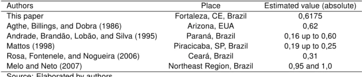
demand. Comparing the estimated values with other papers, the demand elasticity-price is similar to Agthe, Billings, and Dobra (1986) (0,62), Andrade, Brandão, Lobão, and Silva (1995) (0.16 to 0.60); it is higher than those found by Mattos (1998) (0,19 to 0,25), Rosa, Fontenele, and Nogueira (2006) (0,31); and it is lower than Melo and Neto (2007) (0,95 and 1,0). (See, Table 5)

Tabela 5: Demand Price-elasticity in Some Published Papers

Authors Place Estimated value (absolute)

This paper Fortaleza, CE, Brazil 0,6175

Agthe, Billings, and Dobra (1986) Arizona, EUA 0,62 Andrade, Brandão, Lobão, and Silva (1995) Paraná, Brazil 0,16 up to 0,60 Mattos (1998) Piracicaba, SP, Brazil 0,19 up to 0,25 Rosa, Fontenele, and Nogueira (2006) Ceará, Brazil 0,31 Melo and Neto (2007) Northeast Region, Brazil 0,95 and 1,0 Source: Elaborated by authors

When we look at the difference variable, the estimated coefficient of -0,0078 indicates that when there is a increase of R$ 1.00 in the difference between the price that the consumer pays and the price that he/she would pay if all units were charged by the marginal price, consumption decreases by 0.78% on average, once the consumer is paying more than he/she would pay in marginal price.The coefficient estimated of 0.0482 for income means that consumers go from a lower income class to a superior income class, with no changes in his tax status, his consumption increases 4.82%, in ave-rage. Finally, the coefficient estimated of 0.0763 and 0.0415 for total of residents and total of rooms, respectively, indicate a increase of 7.63% and 4.15% in the amount of water consumed when there is a new person in the house and there is a new room. The R2 equals to 0.513 shows a good level of explanatory power for the water demand estimation in a cross-section microdata regression, once the variables used in the model explains 51% in water consumption variation.

Since there is room for spatial dependence on water consumption, we run the Moran-I test for the residues estimated by OLS. The results are presented in table 6. Table 6 shows that the Moran-I statistic is equal to 0.0231 and it is significant. This means that the probability for the spatial association pattern being random is close to zero, supporting the hypothesis of residues spatially dependent. Moreover, the positive value indicates that the autocorrelation is positive, as expected.

Tabela 6: Moran-I statistic for the residues estimated by OLS Moran-I statistic Mean Variance p-value

0,0170 -0,0004 6.72e-06 <_7.39e-12 Source: Elaborated by authors

Note: empirical p-value based on randomization method

there is spatial autocorrelation in the dependent variable. Table 7 presents the results from these tests.

Tabela 7: Lagrange multipliers tests

Test Estimated value df p-value LMλ 40.6957 1 1.77e-10 LMρ 36.9793 1 1.19e-09 RLMλ 10.8584 1 0.0009 RLMρ 7.1419 1 0.0075 SARMA 47.8376 2 4.094e-11 Source: Elaborated by authors

Following the methods proposed by Florax, Folmer, and Rey (2003), we compare the LMλ and LMρ values first. The values of 40.69 and 36.97, both significant, indicates that there is spatial dependence associated both to lag in the dependent variable and to non modeled effects, this last represented by error term. Next, comparing the values for RLMλ and RLMρ we have that both are significant. Also, since RLMλ> RLMρthis indicates that the most appropriate model would be the SEM model.

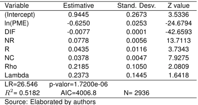
However, since there is spatial autocorrelation both for residues and for the dependent variable, it is possible that the correct model might be the SARMA model. Thus, analyzing the result from the SARMA test shown in table 7, we can see that the value of 47.83 is statistically significant. This implies that the SARMA model is the most appropriated to model spatial effect over residential water demand in the city of Fortaleza. Based on this, we estimated the SARMA model and its results are presented next4_.

Tabela 8: Water Demand (ln) with Spatial Effect - SARMA

Variable Estimative Stand. Desv. Z value (Intercept) 0.9445 0.2673 3.5336 ln(PME) -0.6250 0.0253 -24.6794

DIF -0.0077 0.0001 -42.6593

NR 0.0778 0.0056 13.7113

R 0.0435 0.0116 3.7343

NC 0.0378 0.0047 7.9275

Rho 0.2185 0.1050 2.0809

Lambda 0.2373 0.1445 1.6418

LR=26.546 p-valor=1.7200e-06 R2

= 0.5182 AIC=4006.8 N= 2936 Source: Elaborated by authors

The results presented in Table 8 show that the estimated coefficient of autoregressive parameters linked to both the lagged dependent variable and the error term are statistically significant