Pricing Dual Spread Options by the Lie-Trotter
Operator Splitting Method
C.F. Lo
Abstract—In this paper, based upon the Lie-Trotter operator splitting method proposed by Lo (2014), we present a simple closed-form ap-proximation for pricing the (three-asset) dual spread options. Illustrative numerical exam-ples show that the proposed approximation is not only extremely fast and robust, but also it is very accurate for typical volatilities and maturities up to two years. Moreover, for the case of a vanishing strike the proposed approx-imation becomes exact.
Keywords: Spread options; Kirk’s approximation; Lie-Trotter operator splitting method
I. INTRODUCTION
A spread option is an option whose payo¤ is linked to the price di¤erence of two underlying as-sets and forms the simplest type of multi-asset op-tions. Spread options are very popular in interest rate markets, currency and foreign exchange mar-kets, commodity marmar-kets, and energy markets nowa-days.[1] Unlike pricing single-asset options, pricing spread options is a very challenging task. The major di¢culty stems from the lack of knowledge about the distribution of the spread of two correlated lognormal random variables. The simplest approach is to eval-uate the expectation of the …nal payo¤ over the joint probability distribution of the two correlated lognor-mal underlyings by means of numerical integration. However, practitioners often prefer to use analyti-cal approximations rather than numerianalyti-cal methods because of their computational ease. Among vari-ous analytical approximations, Kirk’s approximation seems to be the most popular and is the current mar-ket standard, especially in the energy marmar-kets.[2] It Author for correspondence. Institute of Theoretical Physics and Department of Physics, The Chinese University of Hong Kong, Shatin, New Territories, Hong Kong (Email: c‡[email protected])
is well known that Kirk’s approximation extends from Margrabe’s exchange option formula with no rigorous derivation.[3] Recently, Lo (2013) applied the idea of WKB method to provide a derivation of Kirk’s ap-proximation and discuss its validity.[4] Nevertheless, it is not straightforward to apply Lo’s approach either to provide a generalization of Kirk’s approximation for the multi-asset case or to improve Kirk’s approx-imation while retaining its favourable features.
In order to overcome these shortcomings, Lo (2014) subsequently presented a simple uni…ed ap-proach,[5,6] namely the Lie-Trotter operator splitting method,[7-12] not only to rigorously derive Kirk’s ap-proximation but also to obtain a generalization for the case of multi-asset spread option in a straightforward manner. The derived price formula for the multi-asset spread option bears a striking resemblance to Kirk’s approximation in the two-asset case. Illustra-tive numerical examples have demonstrated that the multi-asset generalization retains all the favourable features of Kirk’s approximation. More importantly, the proposed approach is able to provide a new per-spective on Kirk’s approximation and the general-ization; that is, they are simply equivalent to the Lie-Trotter operator splitting approximation to the Black-Scholes equation.
It is the aim of this communication to ap-ply the Lie-Trotter operator splitting method pro-posed by Lo (2014) to derive a closed-form ap-proximate price formula for the (three-asset) dual spread options,[5,6] whose …nal payo¤ has the form
max (S1 S3 K; S2 S3 K;0)withSi being the
shown to demonstrate both the accuracy and e¢-ciency of the proposed approximation. Furthermore, it should be noted that for K = 0 the proposed ap-proximation becomes exact.
II. PRICING DUAL SPREAD OPTIONS BY LIE-TROTTER SPLITTING APPROXIMATION
To price a European three-asset dual call spread option, we need to solve the three-dimensional Black-Scholes equation
3
X
i;j=1
1
2 ij i jFiFj @2
P(F1; F2; F3; )
@Fi@Fj
= @P(F1; F2; F3; )
@ (1)
subject to the …nal payo¤ condition
P(F1; F2; F3;0)
= max (F1 F3 K; F2 F3 K;0) ; (2)
whereFi is the future price of the underlying asseti
with the volatility i, ij is the correlation between
the assets iandj,K is the strike price, and is the time-to-maturity.
Main result:
The price of the dual call spread option can be approximated by
P(F1; F2; F3; )
e r [F
1fN( 1) N2( 1; 2; 1)g
(F3+K)N2 1 ~1
p
; 3; 1 +
F2 N( 4) N2 4; 2 ~
p
; 2
(F3+K)N2 4 ~2
p
; 3; 2 : (3)
where
1 =
ln (F1=[F3+K]) + 1 2~
2 1
~1p
2 =
ln (F2=F1) 1 2~
2
~ p
3 =
ln (F1=F2) 1 2 ~
2 1 ~
2 2
~ p
4 =
ln (F2=[F3+K]) + 1 2~
2 2
~2p 1 =
~12~2 ~1
~
2 =
~12~1 ~2
~
~ =
q ~2
1 2~12~1~2+ ~ 2 2
~1 =
q
2
1 2 13 1~3+ ~ 2 3
~2 =
q
2
2 2 23 2~3+ ~ 2 3
~3 = 3
F3
F3+K
~12 =
12 1 2 ( 13 1+ 23 2 ~3) ~3
~1~2
(4)
andN2( )is the cumulative bivariate normal
distrib-ution function.
Derivation:
In terms of the new variables
R1=
F1
F3+K
; R2=
F2
F3+K
; R3=F3+K (5)
we can express Eq.(1) as n
^
L0+ ^L1+ ^L2 r
o
P(R1; R2; R3; )
= @P(R1; R2; R3; )
@ ; (6)
where ^ L0 =
1 2~
2 1R
2 1
@2
@R2 1
+1
2~
2 2R
2 2
@2
@R2 2
+
~12~1~2R1R2
@2
@R1@R2
^
L1 = ( 13 1 ~3) ~3R1R3
@2
@R1@R3
( 13 1 ~3) ~3R1
@ @R1
+1 2~
2 3R
2 3
@2
@R2 3
^
L2 = ( 23 2 ~3) ~3R2R3
@2
@R2@R3
( 23 2 ~3) ~3R2
@ @R2
+1 2~
2 3R
2 3
@2
@R2 3
: (7)
The …nal payo¤ condition now becomes
P(R1; R2; R3;0) =R3max (R1 1; R2 1;0) : (8)
It is obvious that Eq.(6) has the formal solution
P(R1; R2; R3; )
= e r expn L^
0+ ^L1+ ^L2
o
R3max (R1 1; R2 1;0) : (9)
namely (see the Appendix)
PLT(R
1; R2; R3; )
= e r expn L^0
o
expn L^1+ ^L2
o
R3max (R1 1; R2 1;0)
= e r R
3exp
n ^ L0
o
max (R1 1; R2 1;0)
e r R
3C(R1; R2; ) : (10)
Here C(R1; R2; ) satis…es the partial di¤erential
equation
@C(R1; R2; )
@ = 1 2~ 2 1R 2 1 @2 @R2 1
+ ~12~1~2R1R2
@2
@R1@R2
+ 1 2~ 2 2R 2 2 @2 @R2 2
r C(R1; R2; ) (11)
with the initial condition: C(R1; R2; = 0) =
max (R1 1; R2 1;0). Since ~1, ~2 and ~12 are
independent ofR1andR2, we have a problem of
pric-ing a European “best-of-two” option.[13] The desired solution of Eq.(11) is simply given by
C(R1; R2; )
= e r
Z 1
1 dx10
Z 1
1
dx20f(x1; x2; ;x10; x20)
max (ex10
1; ex20 1;0)
= e r
Z 1
0
dx10
Z x10
1
dx20f(x1; x2; ;x10; x20)
(ex10 1) +
e r
Z 1
0
dx20
Z x20
1
dx10f(x1; x2; ;x10; x20)
(ex20
1) (12)
where x10 = lnR10, x20 = lnR20, x1 = lnR1, x2 =
lnR2, and
f(x1; x2; ;x10; x20)
= 1
2 ~1~2
q
1 ~2
12
exp (
1 2~2
1 1 ~ 2 12
x10 x1+
1 2~
2 1
2
+ ~12
~1~2 1 ~
2 12
x10 x1+
1 2~
2 1
x20 x2+
1 2~
2 2
1
2~22 1 ~
2 12
x20 x2+
1 2~ 2 2 2) : (13)
After carrying out the integrals in Eq.(12), the solu-tion can be determined in closed form as follows:
C(R1; R2; )
= e r [R
1fN( 1) N2( 1; 2; 1)g
N2 1 ~1
p
; 3; 1 +
R2 N( 4) N2 4; 2 ~
p
; 2
N2 4 ~2
p
; 3; 2 : (14)
As a result, the approximate solution
PLT(R
1; R2; R3; ) = R3C(R1; R2; ) yields the
approximate price formula given in Eq.(3). In terms of the spot asset prices, namely Si
Fiexp ( r ) , the price formula given in Eq.(3) has
the form
PKirk(S1; S2; S3; )
= S1fN(d1) N2(d1; q; 1)g
S3+Ke r N2(d2; p; 1) +
S2 N(h1) N2 h1; q ~
p
; 2
S3+Ke r N2(h2; p; 2) (15)
where
d1 =
ln (S1=[S3+Ke r ]) + 1 2~
2 1
~1p
d2 = d1 ~1
p
h1 =
ln (S2=[S3+Ke r ]) + 1 2~
2 2
~2p
h2 = h1 ~2
p
p = ln (S1=S2)
1 2 ~ 2 1 ~ 2 2 ~ p
q = ln (S2=S1)
1 2~
2
~ p : (16)
It should be noted that the Lie-Trotter operator splitting approximation is particularly applicable for those dual spread options with short maturities, i.e.
~21 1 and ~
2
2 1. Furthermore, for K = 0,
the operators L^0, L^1 and L^2 commute so that the
Lie-Trotter splitting approximation becomes exact.
III. ILLUSTRATIVE NUMERICAL EXAMPLES In this section illustrative numerical examples are presented to demonstrate the accuracy of the pro-posed approximation for the dual spread options. We examine a simple dual spread option with the …nal payo¤ max (S1 S3 K; S2 S3 K;0). Table I
T. Other input model parameters are set as follows:
r= 0:05, 1= 2 = 3 = 0:3, 12 = 0:2, 23= 0:4, 13 = 0:8, S1 = 150, S2 = 60and S3 = 50. Monte
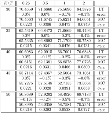
Carlo estimates and the corresponding standard de-viations are also presented for comparison. It is ob-served that the computed errors of the approximate option prices are capped at0:2%(in magnitude). In fact, most of them are less than0:1%. Then, in Table II the e¤ect of increasing the three volatilities (from 0:3 to 0:6) upon the approximate estimation of the option prices is investigated. Obviously only a small increase occurs in the computed errors, and these er-rors are still less than0:7%(in magnitude).
Table I:
Prices of a European dual call spread option. Other input parameters are: r= 0:05, 1= 2 = 3= 0:3, 12= 0:2, 23= 0:4, 13= 0:8,S1 =150, S2 = 60 andS3 = 50. Here “LT” refers to the
proposed approximation based upon the Lie-Trotter operator splitting method while “MC” denotes the Monte Carlo estimates with900;000;000replications. The relative errors of the “LT” option prices with respect to the “MC” estimates are also presented.
KnT 0:25 0:5 1 2
30 70:3727 70:7428 71:5561 73:7670 LT
0:0% 0:0% 0:0% 0:0% error
70:3732 70:7422 71:5578 73:7724 MC
0:0104 0:0168 0:0227 0:0333 M C
35 65:4348 65:8662 66:8025 69:2787 LT
0:0% 0:0% 0:0% 0:0% error
65:4351 65:8669 66:8025 69:2917 MC
0:0119 0:0168 0:0215 0:0334 M C
40 60:4969 60:9899 62:0562 64:8309 LT
0:0% 0:0% 0:0% 0:1% error
60:4971 60:9899 62:0581 64:8664 MC
0:0107 0:0160 0:0220 0:0324 M C
45 55:5590 56:1146 57:3291 60:4500 LT
0:0% 0:0% 0:0% 0:1% error
55:5585 56:1165 57:3421 60:5071 MC
0:0110 0:0147 0:0228 0:0301 M C
50 50:6212 51:2440 52:6426 56:1672 LT
0:0% 0:0% 0:1% 0:2% error
50:6213 51:2469 52:6677 56:2557 MC
0:0108 0:0140 0:0200 0:0303 M C
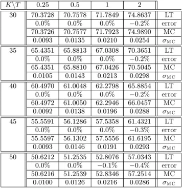
Finally, we study a case in which all the three volatilities are di¤erent, namely 1 = 0:3, 2 = 0:4
and 3 = 0:5, while the other parameters remain
the same. According to Table III, the computed er-rors are generally reduced a little bit in this case and they do not exceed0:4%(in magnitude). Moreover,
since the approximate option price formula is given in closed form, its evaluation is instantaneous. As a result, it can be concluded that the proposed closed-form approximation for the dual spread options are found to be very accurate and e¢cient.
IV. CONCLUSION
In this paper, based upon the Lie-Trotter oper-ator splitting method proposed by Lo (2014),[5,6] we have presented a simple closed-form approxima-tion for pricing the (three-asset) dual spread opapproxima-tions. The derived price formula bears a close resemblance to that of a European “best of two” option. As demonstrated by illustrative numerical examples for the dual spread options, the proposed approximation is not only extremely fast and robust, but also it is very accurate for typical volatilities and maturities of up to two years. Moreover, for the case of a vanish-ing strike, i.e. K = 0, the proposed approximation becomes exact.
Table II:
Prices of a European dual call spread option. Other input parameters are: r= 0:05, 1= 2= 3= 0:6, 12= 0:2, 23= 0:4, 13= 0:8,S1 =150, S2 = 60 andS3 = 50. Here “LT” refers to the
proposed approximation based upon the Lie-Trotter operator splitting method while “MC” denotes the Monte Carlo estimates with900;000;000replications. The relative errors of the “LT” option prices with respect to the “MC” estimates are also presented.
KnT 0:25 0:5 1 2
30 70:4659 71:6660 75:5696 84:3876 LT
0:0% 0:0% 0:1% 0:3% error
70:4663 71:6745 75:6231 84:6051 MC
0:0223 0:0306 0:0473 0:0749 M C
35 65:5319 66:8473 71:0669 80:4493 LT
0:0% 0:0% 0:2% 0:4% error
65:5335 66:8692 71:1709 80:7580 MC
0:0215 0:0341 0:0476 0:0731 M C
40 60:6083 62:0915 66:7001 76:6848 LT
0:0% 0:1% 0:2% 0:5% error
60:6151 62:1381 66:8578 77:0725 MC
0:0216 0:0331 0:0466 0:0800 M C
45 55:7114 57:4357 62:5004 73:1061 LT
0:0% 0:1% 0:3% 0:6% error
55:7275 57:5148 62:7155 73:5664 MC
0:0221 0:0320 0:0391 0:0658 M C
50 50:8689 52:9202 58:4926 69:7183 LT
0:1% 0:2% 0:5% 0:7% error
50:8995 53:0358 58:7584 70:2351 MC
Table III:
Prices of a European dual call spread option. Other input parameters are: r= 0:05, 1=0:3, 2 = 0:4, 3 = 0:5, 12 = 0:2, 23 = 0:4, 13 =
0:8, S1 = 150, S2 = 60 and S3 = 50. Here “LT”
refers to the proposed approximation based upon the Lie-Trotter operator splitting method while “MC” de-notes the Monte Carlo estimates with 900;000;000 replications. The relative errors of the “LT” option prices with respect to the “MC” estimates are also presented.
KnT 0:25 0:5 1 2
30 70:3728 70:7578 71:7849 74:8637 LT
0:0% 0:0% 0:0% 0:2% error
70:3726 70:7577 71:7923 74:9890 MC
0:0093 0:0135 0:0210 0:0254 M C
35 65:4351 65:8813 67:0308 70:3651 LT
0:0% 0:0% 0:0% 0:2% error
65:4351 65:8810 67:0426 70:5045 MC
0:0105 0:0143 0:0213 0:0298 M C
40 60:4970 61:0048 62:2798 65:8854 LT
0:0% 0:0% 0:0% 0:2% error
60:4972 61:0050 62:2946 66:0457 MC
0:0092 0:0138 0:0196 0:0288 M C
45 55:5591 56:1286 57:5358 61:4321 LT
0:0% 0:0% 0:0% 0:3% error
55:5597 56:1302 57:5556 61:6195 MC
0:0093 0:0146 0:0191 0:0293 M C
50 50:6212 51:2535 52:8076 57:0343 LT
0:0% 0:0% 0:1% 0:4% error
50:6216 51:2539 52:8346 57:2514 MC
0:0100 0:0126 0:0216 0:0286 M C
APPENDIX:
Suppose that one needs to exponentiate an oper-ator C^ which can be split into two di¤erent parts, namelyA^and B^. For simplicity, let us assume that
^
C= ^A+ ^B, where the exponential operator exp ^C
is di¢cult to evaluate butexp A^ andexp B^ are either solvable or easy to deal with. Under such cir-cumstances the exponential operatorexp "C^ , with
" being a small parameter, can be approximated by the Lie-Trotter operator splitting formula:[7-12]
exp "C^ = exp "A^ exp "B^ +O "2
: (A.1) The Lie-Trotter splitting approximation is particu-larly useful for studying the short-time behaviour of the solutions of evolutionary partial di¤erential equa-tions of parabolic type because for this class of prob-lems it is sensible to split the spatial di¤erential op-erator into several parts each of which corresponds to
a di¤erent physical contribution (e.g., reaction and di¤usion).
REFERENCES:
[1] Carmona, R. and Durrleman, V., “Pricing and hedg-ing spread options”, SIAM Review, vol.45, no.4, pp.627-685 (2003).
[2] Kirk, E., “Correlation in the Energy Markets” in Managing Energy Price Risk (1995).
[3] Margrabe, W., “The value of an option to exchange one asset for another”, Journal of Finance, vol.33, pp.177-186 (1978).
[4] Lo, C.F., “A simple derivation of Kirk’s approxima-tion for spread opapproxima-tions”, Applied Mathematics Let-ters, vol.26, no.8, pp.904-907 (2013).
[5] Lo, C.F., “A simple generalisation of Kirk’s approx-imation for multi-asset spread options by the Lie-Trotter operator splitting sethod”,Journal of Math-ematical Finance, vol.4, no.3, pp.178-187 (2014).
[6] Lo, C.F., “Valuing multi-asset spread options by the Lie-Trotter operator splitting method”, Lecture Notes in Engineering and Computer Science: Pro-ceedings of The World Congress on Engineering 2014 (2-4 July, 2014, London, U.K.), pp.911-915 (2014).
[7] Trotter, H.F., “On the Product of Semi-Groups of Operators”,Proceedings of the American Math. So-ciety, vol.10, no.4, pp.545-551 (1959).
[8] Trotter, H.F., “Approximation of semi-groups of op-erators”,Paci…c J. Math., vol.8, pp.887-919 (1958).
[9] Suzuki, M., “Decomposition formulas of exponential operators and Lie exponentials with some applica-tions to quantum mechanics and statistical physics”, J. Math. Phys., vol.26, no.4, pp.601-612 (1985).
[10] Drozdov, A.N. and Brey, J.J., “Operator expansions in stochastic dynamics”,Phy. Rev. E, vol.57, no.2, pp.1284-1289 (1998).
[11] Hatano, N. and Suzuki, M., “Finding exponential product formulas of higher orders”, Lect. Notes Phys., vol.679, pp.37-68 (2005).
[12] Blanes, S., Casas, F., Chartier, P. and Murua, A., “Optimized higher-order splitting methods for some classes of parabolic equations”,Mathematics of Computation, vol.82, no.283, pp.1559-1576 (2013).