A web-based software tool to estimate unregulated daily streamflow at ungauged rivers

(1)

GMDD

5, 2503–2526, 2012

A web-based software tool to estimate unregulated

daily streamflow

S. A. Archfield et al.

Title Page Abstract Introduction Conclusions References

Tables Figures

◭ ◮

Back Close

Full Screen / Esc

Printer-friendly Version Interactive Discussion

Discussion

P

a

per

|

Dis

cussion

P

a

per

|

Discussion

P

a

per

|

Discussio

n

P

a

per

|

Geosci. Model Dev. Discuss., 5, 2503–2526, 2012 www.geosci-model-dev-discuss.net/5/2503/2012/ doi:10.5194/gmdd-5-2503-2012

Geoscientific Model Development Discussions

This discussion paper is/has been under review for the journal Geoscientific Model Development (GMD). Please refer to the corresponding final paper in GMD if available.

A web-based software tool to estimate

unregulated daily streamflow at ungauged

rivers

S. A. Archfield1, P. A. Steeves1, J. D. Guthrie2, and K. G. Ries III3

1

Massachusetts-Rhode Island Water Science Center, US Geological Survey, 10 Bearfoot Road, Northborough, MA 01532, USA

2

Rocky Mountain Geographic Science Center, US Geological Survey, P.O. Box 25046 MS 516, Denver Federal Center, Denver, CO 80225, USA

3

Office of Surface Water, US Geological Survey, 5522 Research Park Drive, Baltimore,

Maryland 21228, USA

Received: 24 July 2012 – Accepted: 9 August 2012 – Published: 31 August 2012

Correspondence to: S. A. Archfield (sarch@usgs.gov)

(2)

GMDD

5, 2503–2526, 2012

Tables Figures

◭ ◮

Back Close

Full Screen / Esc

Discussion

P

a

per

|

Dis

cussion

P

a

per

|

Discussion

P

a

per

|

Discussio

n

P

a

per

|

Abstract

Streamflow information is critical for solving any number of hydrologic problems. Often times, streamflow information is needed at locations which are ungauged and, there-fore, have no observations on which to base water management decisions. Further-more, there has been increasing need for daily streamflow time series to manage rivers

5

for both human and ecological functions. To facilitate negotiation between human and ecological demands for water, this paper presents the first publically-available, map-based, regional software tool to interactively estimate daily streamflow time series at any user-selected ungauged river location. The map interface allows users to locate and click on a river location, which then returns estimates of daily streamflow for the

10

location selected. For the demonstration region in the northeast United States, daily

streamflow was shown to be reliably estimated by the software tool, with efficiency

val-ues computed from observed and estimated streamflows ranging from 0.69 to 0.92. The software tool provides a general framework that can be applied to other regions for which daily streamflow estimates are needed.

15

1 Introduction

Streamflow information at ungauged rivers is needed for any number of hydrologic applications; this need is of such importance that an international research initiative known as Prediction in Ungaged Basins (PUB) has been underway for the past decade (Sivapalan et al., 2003). Concurrently, there has been increasing emphasis on the need

20

for daily streamflow time series to understand the complex response of ecology to river regulation and to develop streamflow prescriptions to restore and protect aquatic

habi-tat (Po_ffet al., 1997, 2010). Basin-wide water allocation decisions that meet both

hu-man and ecological dehu-mands for water require daily streamflow time series at river locations that have ecological constraints on water (locations where important or

pro-25

(3)

GMDD

5, 2503–2526, 2012

Tables Figures

◭ ◮

Back Close

Full Screen / Esc

Discussion

P

a

per

|

Dis

cussion

P

a

per

|

Discussion

P

a

per

|

Discussio

n

P

a

per

|

water (locations on the river that are dammed or otherwise managed), or locations that have both constraints. Often times, these locations are unmonitored and no information is available to make informed decisions about water allocation.

Methods to estimate daily streamflow time series at ungauged locations can be broadly characterized under the topic of regionalization (Bl ¨oschl and Sivapalan, 1995),

5

an approach which pools information about streamgauges in a region and transfers this information to an ungauged location. Generally there are two main categories of

information that is pooled and transferred: (1) rainfall-runo_ff model parameters that

are calibrated at gauged catchments and transferred in some way to an ungauged location (see Zhang and Chiew, 2009 for a review) and (2) gauged streamflows, or

10

related streamflow properties, are directly transferred to ungauged locations. Exam-ples of this type of regionalization approach include geostatistical methods such as top-kriging (Skøien and Bl ¨oschl, 2007) and more commonly used methods such as the drainage-area ratio method (as described in Archfield and Vogel, 2010), the MOVE method (Hirsch, 1979), and a non-linear spatial interpolation method, applied by

Fen-15

nessey (1994), Hughes and Smakhtin (1996), Smakhtin (1999), Mohamoud (2008), Archfield et al. (2010), and Shu and Ourda (2012). For the software tool presented in this paper, a hybrid approach combining the drainage-area ratio and non-linear spatial interpolation methods is used to estimate daily streamflow time series.

When streamflow information is presented in an easy-to-use, freely-available

soft-20

ware tool, this information can provide a scientific framework for water-allocation negotiation amongst stakeholders. Software tools to provide streamflow time series at ungauged locations have been previously published for predefined locations on a river; however few – if any – tools currently exist that provide daily streamflow time series at any stream location for which this information is needed. Smakhtin

25

(4)

GMDD

5, 2503–2526, 2012

Tables Figures

◭ ◮

Back Close

Full Screen / Esc

Discussion

P

a

per

|

Dis

cussion

P

a

per

|

Discussion

P

a

per

|

Discussio

n

P

a

per

|

Resources (WATER) to serve daily streamflow information at fixed stream locations in non-karst areas of Kentucky. These existing tools provide valuable streamflow infor-mation; yet, in most cases, at the monthly – not daily – time step and, in all cases, for only predefined locations on a river that may not be coincident with a river location of interest. The US Geological Survey StreamStats tool (Ries and others, 2008) does

5

provide the utility to delineate a contributing area to a user-selected location on a river; however, only streamflow statistics – not streamflow time series – are provided for the ungauged location.

The software tool presented here is one of the first such tools to provide daily stream-flow time series at ungauged locations in a regional framework for any user-desired

10

location on a river. The software tool has a map-based user interface and leverages recently published methods to estimate daily streamflow at ungauged river locations. This paper first briefly describes the methods used by the software tool. The software tool is then presented and its functionality is described. Lastly the utility of the software tool to provide reliable estimates of daily streamflow is demonstrated for a large basin

15

in the northeast United States.

2 Methods underlying the software tool

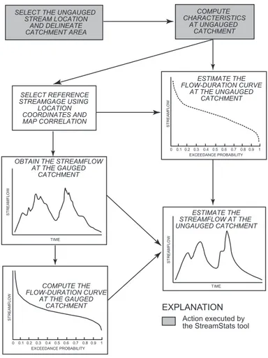
Streamflow is estimated in the software tool using information from an index stream-gauge and catchment characteristics computed for the contributing area to the un-gauged stream location of interest (Fig. 1). Catchment characteristics and the selected

20

index streamgauge are first used to estimate a continuous, daily flow-duration curve (FDC) at the ungauged location (Fig. 1). The estimated FDC is then transformed to a time series of streamflow values by the index streamgauge (Fig. 1). The methods to estimate the FDC, select the index streamgauge, and transform the FDC to a time series of daily streamflow are explained in detail in the following sections.

(5)

GMDD

5, 2503–2526, 2012

Tables Figures

◭ ◮

Back Close

Full Screen / Esc

Discussion

P

a

per

|

Dis

cussion

P

a

per

|

Discussion

P

a

per

|

Discussio

n

P

a

per

|

2.1 Estimation of the flow-duration curve for the ungauged location

Estimation of the daily FDC at an ungauged location remains an outstanding challenge in hydrology. Castellarin et al. (2004) provides a review of several methods to estimate FDCs at ungauged locations and found that no particular method was consistently better than another. For this study, an empirical, piece-wise approach to estimate the

5

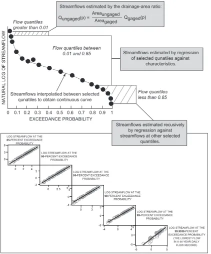
FDC is used in the software tool (Fig. 2). This overall approach is similar to that used by Mohamoud (2008), Archfield et al. (2010), and Shu and Ourda (2012) in that the FDC is estimated by first developing regional regressions relating catchment characteristics to selected FDC quantiles and then interpolating between those quantiles to obtain a continuous FDC.

10

With the exception of streamflows having less than or equal to a 0.01 probability of being exceeded (streamflows with a probability of being exceeded more than 1 per-cent of the time), selected quantiles on the FDC are estimated from regional regression equations and a continuous FDC is log-linearly interpolated between these quantiles to obtain a continuous FDC (Fig. 2). Relations between streamflow quantiles at the 0.02,

15

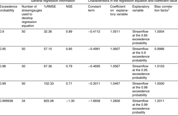
0.05, 0.1, 0.15, 0.2, 0.25, 0.3, 0.4, 0.5, 0.6, 0.7, 0.75, 0.8 and 0.85 exceedance prob-abilities were estimated by independently regressing each streamflow quantile against catchment characteristics (Fig. 2). Following the approach in Archfield et al. (2010), relations between streamflow quantiles at the 0.9, 0.95, 0.98, 0.99 and 0.999938 were estimated by regressing streamflows at these quantiles against one another and using

20

these relations to recursively estimate streamflows (Fig. 2). Recursively estimating low streamflows, as was done in Archfield et al. (2010), exploits the strong structural rela-tion between the streamflow quantiles (Fig. 2) and enforces the constraint that stream-flows must decrease as the exceedance probability increases. Mohamoud (2008) and Archfield et al. (2010) observed that when regression is done against catchment

char-25

(6)

GMDD

5, 2503–2526, 2012

Tables Figures

◭ ◮

Back Close

Full Screen / Esc

Discussion

P

a

per

|

Dis

cussion

P

a

per

|

Discussion

P

a

per

|

Discussio

n

P

a

per

|

Regressing quantiles against one another ensures that this constraint is not violated. This is an alternative approach to that used by Mohamoud (2008), who suggested discarding any estimated quantiles that violate the constraint. All regressions were fit using methods outlined in Archfield et al. (2010).

Archfield et al. (2010) showed that estimated streamflows determined by log-linear

5

interpolation for exceedance probabilities of 0.01 or less do not match the shape of the FDC in this range and this interpolation method creates a bias in the estimated streamflows, which can substantially overestimate the peak streamflows. The shape of the FDC at the highest streamflows is so complex that, instead of using another interpolation method, streamflows from an index streamgauge are scaled to estimate

10

the highest streamflows at the ungauged location. The assumption here is that the shape of the left tail of the FDC is better approximated by the streamflow quantiles at an index streamgauge than by a curve fit. Therefore, for streamflows having less than or equal to a 0.01 probability of being exceeded, streamflows are scaled by a drainage-area ratio approach (Eq. 1) in conjunction with the selected index streamgauge:

15

q_p

u =

A_u

A_gqpg (1)

where q_p

u is the value of the streamflow quantile at the ungauged location for

ex-ceedance probability,p,A_uis the contributing drainage area to the ungauged location,

A_g is the contributing drainage area to the index streamgauge, andq_p

g is the value of

the streamflow quantile at the index streamgauge for exceedance probability,p.

20

2.2 Selection of the index streamgauge

As shown in Fig. 1, the index streamgauge is used for two purposes in the stream-flow estimation approach: (1) to estimate streamstream-flows that have less than a 1-percent chance of being exceeded, and (2) to transform the estimated FDC into a time se-ries of streamflow at the ungauged location. The index streamgauge is selected by the

(7)

GMDD

5, 2503–2526, 2012

Tables Figures

◭ ◮

Back Close

Full Screen / Esc

Discussion

P

a

per

|

Dis

cussion

P

a

per

|

Discussion

P

a

per

|

Discussio

n

P

a

per

|

map-correlation method (Archfield and Vogel, 2010). The map-correlation method se-lects the index streamgauge estimated to have the highest cross-correlation between streamflow time series at the index streamgauge and the ungauged location. Archfield and Vogel (2010) showed that the selection of the index streamgauge using cross-correlation between streamflow time series outperformed the selection of the nearest

5

index streamgauge when used with the drainage-area ratio method to estimate daily streamflow time series at ungauged locations. This finding supports the use of the map-correlation method for two reasons: (1) the drainage-area ratio approach is also used to estimate streamflows that have less than a 1-percent chance of being exceeded, and (2) because the streamflow time series is constructed by transferring the timing

10

of the streamflows at an index streamgauge to the ungauged location, it follows that one would seek to select the index streamgauge that maximizes the cross-correlation between the streamflows at the ungauged location and the index streamgauge. Details of the map correlation method are described in Archfield and Vogel (2010).

2.3 Generation of streamflow time series

15

With an index streamgauge and estimated daily FDC at the ungauged location, a time series of daily streamflow for the simulation period is then constructed by use of the QPPQ transform method (Fennessey, 1994; Hughes and Smakhtin , 1996; Smakhtin, 1999; Mohamoud, 2008; Archfield et al. 2010; Shu and Ourda, 2012). The term QPPQ-transform method was coined by Fennessey (1994); however, this method has been

20

by published Smakhtin (1999), Mohamoud (2008), and Archfield et al. (2010) under names including “non-linear spatial interpolation technique” (Hughes and Smakhtin,

1996; Smakhtin, 1999) and “reshuffling procedure” (Mohamoud, 2008). The method

assumes that the exceedance probability associated with a streamflow on a given day at the index streamgauge also occurred on the same day as the ungauged location.

25

(8)

GMDD

5, 2503–2526, 2012

Tables Figures

◭ ◮

Back Close

Full Screen / Esc

Discussion

P

a

per

|

Dis

cussion

P

a

per

|

Discussion

P

a

per

|

Discussio

n

P

a

per

|

QPPQ-transform method in the software tool, a FDC is constructed from the observed streamflows at the index streamgauge, and then the FDC and the daily flow time se-ries are used together to construct a daily time sese-ries of exceedance probabilities for the streamgauge. The exceedance probability for each day at the streamgauge is then entered sequentially into the estimated FDC for the ungauged location to construct the

5

daily streamflow time series there.

3 Software tool

All data underlying the software tool and methods are freely available across the United States and, therefore, the software tool can be considered a general framework to pro-vide daily streamflow time series at ungauged locations in other regions. The software

10

tool initially interfaces with the US Geological Survey StreamStats tool (Ries et al., 2008) to delineate a catchment area for any user-selected location on a river and to compute the catchment characteristics needed to estimate the FDC at the ungauged location (Fig. 1). The selection of the index streamgauge, the computation of the FDC and the estimate of the time series of daily streamflow is executed by a Microsoft

Ex-15

cel spreadsheet program with Visual Basic for Applications (VBA) coding language. The spreadsheet itself, which contains the VBA source code, can be used indepen-dently of the StreamStats interface and is, therefore, able to be customized to interface with other watershed delineation tools or with any study area for which the methods in Sect. 2 have been applied.

20

The StreamStats tool operates within a web browser, and is accessible at http:// streamstats.usgs.gov. The StreamStats home page provides a general description of the application. A gray box on the left side of the page contains a series of links to pages that document how to use the application, define terminology, and so forth. The map navigation tools provided in the StreamStats user interface should be used to

25

(9)

GMDD

5, 2503–2526, 2012

Tables Figures

◭ ◮

Back Close

Full Screen / Esc

Discussion

P

a

per

|

Dis

cussion

P

a

per

|

Discussion

P

a

per

|

Discussio

n

P

a

per

|

of interest. With the map zoomed into a scale of at least 1:24,000, pressing on the

Watershed Delineation button, and then on the map at location of interest will cause

the catchment boundary for the selected location to be delineated and displayed on the

map (Fig. 3A). Once the catchment is delineated, pressing on theBasin Characteristics

button will result in the appearance of a new browser window that contains a table of

5

the catchment characteristics for the selected location (Fig. 3B). StreamStats uses the

processes described byESRI, Inc.(2012) for catchment delineation and computation

of catchment characteristics. StreamStats also provides a Download tool to export a

shapefile of the contributing catchment (Fig. 5A) for use in other mapping applications. The Microsoft Excel spreadsheet used to estimate daily streamflow for the stream

10

location of interest contains five worksheets (Figs. 3C–F). The spreadsheet opens on

the MainMenu worksheet, which provides additional instruction and support contact

information (Fig. 3C). The user enters the catchment characteristics summarized by

StreamStats into theBasinCharacteristics worksheet (Fig. 3D) and then presses the

command button to compute the unregulated daily streamflows. The program then

fol-15

lows the process outlined in Fig. 1 and Sect. 2. The estimated streamflows are, in part, computed from regional regression equations that were developed using the catch-ment characteristics from the approach discussed in Sect. 2.1. Streamflows estimated for ungauged catchments having characteristics outside the range of values used to develop the regression equations are highly uncertain because these values were not

20

used to fit the regression equations. Therefore, the software tool includes a message in

theBasinCharacteristicsworksheet (Fig. 3D) next to each characteristic that is outside

the respective ranges of those characteristics used to solve the regression equations.

The ReferenceGaugeSelection worksheet (Fig. 3E) displays information about the

ungauged catchment and index streamgauge that was selected from the method

de-25

scribed in Sect. 2.2, including the percent difference between catchment characteristics

(10)

GMDD

5, 2503–2526, 2012

Tables Figures

◭ ◮

Back Close

Full Screen / Esc

Discussion

P

a

per

|

Dis

cussion

P

a

per

|

Discussion

P

a

per

|

Discussio

n

P

a

per

|

selects the index streamgauge estimated to be most correlated with the ungauged location, the five index streamgauges estimated to be most correlated with the un-gauged location are also reported (Fig. 3E). The tool also allows users to choose from any of the potential index streamgauges in the study (Fig. 3E). Users select a new index streamgauge from a pull-down list and then choose the update button (Fig. 3E).

5

The ContinuousFlowDuration worksheet (Fig. 3F) displays the estimated continuous

exceedance probabilities, and theContinuousDailyFlow worksheet (Fig. 3G) displays

the estimated daily time series for the ungauged site.

3.1 Demonstration area

The methods described in Sect. 2 were applied to the Connecticut River Basin (CRB),

10

located in the northeast United States, and incorporated into a basin-specific tool termed the Connecticut River UnImpacted Streamflow Estimator (CRUISE) tool. The CRUISE tool is freely available for download at http://webdmamrl.er.usgs.gov/s1/sarch/ ctrtool/index.html. The CRB is located in the northeast United States and covers an

area of approximately 29 000 km2(Fig. 1). The region is characterized by a temperate

15

climate with distinct seasons. Snowfall is common from December through March, with generally more snow falling in the northern portion of the CRB than in the south. The

geology and hydrology of the study region are heavily affected by the growth and retreat

of glaciers during the last ice age, which formed the present-day stream network and drainage patterns (Armstrong et al., 2008). The retreat of the glaciers filled the river

20

valleys with outwash sands and gravel as well as fine- to coarse-grained lake deposits (Armstrong et al., 2008), and these sand and gravel deposits have been found to be important controls on the magnitude and timing of base flows in the southern portion of the study region (Ries and Friesz, 2000). The CRB has thousands of dams along the mainstem and tributary rivers that are used for hydropower, flood control, and water

25

(11)

GMDD

5, 2503–2526, 2012

Tables Figures

◭ ◮

Back Close

Full Screen / Esc

Discussion

P

a

per

|

Dis

cussion

P

a

per

|

Discussion

P

a

per

|

Discussio

n

P

a

per

|

streamflow time series at ungauged locations to understand how dam management can be optimized to meet both human and ecological needs for water.

Data from streamgauges located within the CRB and surrounding area are used in the CRUISE tool to estimate daily streamflow time series at ungauged locations (Ta-ble 1). The study streamgauges have at least 20 yr of daily streamflow record and

5

have minimal regulation in the contributing catchment to the streamgauge (Armstrong et al., 2008; Falcone et al., 2010). Previous work in the southern portion of the study area by Archfield et al. (2010) showed that the contributing area to the streamgauge, percent of the contributing area with surficial sand and gravel deposits, and mean an-nual precipitation values for the contributing area are important variables in modeling

10

streamflows at ungauged locations. For this reason, these characteristics were sum-marized for the study streamgauges and used in the streamflow estimation process.

Contributing area to the study streamgauges ranges from 0.5 km2to 1845 km2 with a

median value of 200 km2. Mean annual precipitation ranges from 101 cm per year to

157 cm per year with a median value of 122 cm per year. Percent of the contributing

15

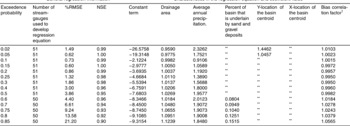
area with surficial sand and gravel ranges from 0 percent to 67 percent with a median value of 9.5 percent. Streamflow in the CRUISE tool is estimated for a 44-yr daily period spanning 1 October 1960 through 30 September 2004 using the methods described in

Sect. 2. Estimated regression coefficients and variogram model parameters are shown

in Tables 2–4, respectively.

20

3.2 Performance of estimated streamflows

To evaluate the utility of the underlying methods to estimate unregulated, daily stream-flow at ungauged locations, a leave-one-out cross validation for 31 streamgauges (Fig. 4) was applied in conjunction with the methods described in Sect. 2. Goodness of fit between observed and estimated streamflows for the entire simulation period was

25

evaluated using the Nash-Sutcliffe efficiency value (Nash and Sutcliffe, 1970), which

(12)

GMDD

5, 2503–2526, 2012

Tables Figures

◭ ◮

Back Close

Full Screen / Esc

Discussion

P

a

per

|

Dis

cussion

P

a

per

|

Discussion

P

a

per

|

Discussio

n

P

a

per

|

of the observed and estimated streamflows were taken to scale the daily streamflow values so that the high and low streamflow values were more equally weighted in the

calculation of the efficiency metric. Efficiency values were mapped to determine if there

was any spatial bias in the model performance (Fig. 4B). Selected hydrographs were

also plotted to visualize the interpretation of the e_fficiency values (Figs. 4C–E).

5

The values in Fig. 4 show that the streamflows estimated by the CRUISE tool gener-ally have good agreement with the observed streamflows at the 31 validation

stream-gauges. The minimum e_fficiency computed from the transformed daily streamflows is

0.69 and the maximum value is 0.92 (Fig. 4A), with an efficiency value equal to 1

indicting perfect agreement between the observed and estimated streamflows. The

10

e_fficiency values for the untransformed observed and estimated streamflows range

from 0.04 to 0.92 (Fig. 4A). This decrease in efficiency between the transformed and

untransformed observed and estimate streamflows suggest that the fit between the observed and estimated streamflows from the CRUISE tool at high streamflow val-ues is more of a challenge than the fit at the other streamflow valval-ues. Despite this,

15

the CRUISE tool appears to result in high efficiency values across all validation sites

(Fig. 4). Streamgauges in the northern portion of the basin have lower efficiency

val-ues than streamgauges in the middle and southern portions of the basin; however, it should be noted from the hydrographs in Fig. 4 that the CRUISE tool is able to repre-sent the daily features of the hydrographs at the validation streamgauges even though

20

the efficiency values are relatively lower in the northern portion of the study area. The

efficiency values and hydrograph comparisons demonstrate that the CRUISE tool can

provide a reasonable representation of natural streamflow time series at ungauged catchments in the basin.

4 Summary and conclusions

25

(13)

GMDD

5, 2503–2526, 2012

Tables Figures

◭ ◮

Back Close

Full Screen / Esc

Discussion

P

a

per

|

Dis

cussion

P

a

per

|

Discussion

P

a

per

|

Discussio

n

P

a

per

|

and requires only an internet connection, a web browser program, and Microsoft Ex-cel version 2000 or higher. Furthermore, the underlying data used to develop the tool and the source code are freely-available and adaptable to other regions of the United States. Daily streamflow is estimated by a four-part process: (1) delineation of the drainage area and computation of the basin characteristics for the ungauged location,

5

(2) selection of an index streamgauge, (3) estimation of the daily flow-duration curve at the ungauged location, and (4) use of the index streamgauge to transfer the flow-duration curve to a time series of daily streamflow. The software tool, when applied to a river basin in the northeastern United States, provided reliable estimates of observed daily streamflows at 31 validation streamgauges across the basin. This software

frame-10

work and underlying methods can be used to develop map-based, daily-streamflow estimates needed for water management decisions at ungauged stream locations for other regions.

Acknowledgements. The authors would like to acknowledge Kimberly Lutz and Colin Apse of The Nature Conservancy, Richard Palmer, Austin Polebitski and Scott Steinschneider of

15

the University of Massachusetts Amherst and Christopher Hatfield, Woodrow Fields, and John Hickey of the US Army Corps of Engineers, for their technical input. The authors would like to also acknowledge John Magee of the New Hampshire Fish and Game Department, who provided valuable review comments on the software tool, Tomas Smieszek of the US Geological Survey for his help with the software website, Jamie Kendall and Melissa Weil for their help in

20

assembling and preparing the data for the CRUISE tool, and Scott Olsen of the US Geological Survey, who provided a list of unimpaired streamgauges located in northern portion of the CRB. This work was funded by the New England Association of Fish and Wildlife Agencies Northeast Regional Conservation Needs Grant number 2007-06 with matching funds from The Nature Conservancy. Any use of trade, product, or firm names is for descriptive purposes only and

25

(14)

GMDD

5, 2503–2526, 2012

Tables Figures

◭ ◮

Back Close

Full Screen / Esc

Discussion

P

a

per

|

Dis

cussion

P

a

per

|

Discussion

P

a

per

|

Discussio

n

P

a

per

|

References

Archfield, S. A. and Vogel, R. M.: Map correlation method: Selection of a reference stream-gage to estimate daily streamflow at unstream-gaged catchments, Water Resour. Res., 46, W10513, doi:10.1029/2009WR008481, 2010.

Archfield, S., Vogel, R., Steeves, P., Brandt, S., Weiskel, P., and Garabedian, S.: The

Mas-5

sachusetts Sustainable-Yield Estimator: A decision-support tool to assess water availability at ungaged sites in Massachusetts, US Geological Survey Scientific Investigations Report 2009-5227, 41 pp. plus CD-ROM, 2010.

Armstrong, D. S., Parker, G. W., and Richards, T. A.: Characteristics and classification of least altered streamflows in Massachusetts, US Geological Survey Scientific Investigations

Re-10

port, 20075291, 113 pp. plus CD–ROM, 2008.

Castellarin, A., Galeati, G., Brandimarte, L., Montanari, A., and Brath, A.: Regional flow-duration curves: reliability for ungauged basins, Adv. Water Resour., 27, 10, 953–965, 2004. ESRI, Inc.: Arc Hydro: GIS for Water Resources, http://www.esri.com/library/fliers/pdfs/

archydro.pdf, 2012.

15

Falcone, J. A., Carlisle, D. M., Wolock, D. M., and Meador, M. R.: GAGES: A stream gage database for evaluating natural and altered flow conditions in the coterminous United States, Ecology, 91, 612, 2010.

Fennessey, N. M.: A hydro-climatological model of daily streamflow for the northeast United States, Ph.D. dissertation, Tufts University, Department of Civil and Environmental

Engineer-20

ing, 1994.

Hirsch, R. Evaluation of some record reconstruction techniques, Water Resour. Res., 15, 6, 1781–1790, ISSN 0043-1397, 1979.

Holtschlag, D. J.: Application guide for AFINCH, analysis of flows in networks of channels) described by NHDPlus, US Geological Survey Scientific Investigations Report 2009-5188,

25

106 pp., 2009.

Hughes, D. A. and Smakhtin, V. U.: Daily flow time series patching or extension: a spatial interpolation approach based on flow duration curves, Hydrolog. Sci. J., 41, 6, 851–871, 1996.

Mahoamoud, Y. M.: Prediction of daily flow duration curves and streamflow for ungauged

cac-30

(15)

GMDD

5, 2503–2526, 2012

Tables Figures

◭ ◮

Back Close

Full Screen / Esc

Discussion

P

a

per

|

Dis

cussion

P

a

per

|

Discussion

P

a

per

|

Discussio

n

P

a

per

|

Nash, J. E. and Sutcliffe, J. V.: River flow forecasting through conceptual models part I – a

discussion of principles, J. Hydrol., 10, 3, 282–290, 1970.

Poff, N. L., Allen, J. D., Bain, M. B., Karr, J. R., Prestagaard, K. L., Richter, B. D., Sparks, R.

E., and Stromberg, J. C.: The natural-flow regime – A paradigm for river conservation and restoration, Bioscience, 47, 769–784, 1997.

5

Poff, N. L., Richter, B., Arthington, A., Bunn, S. E., Naiman, R. J., Kendy, E., Acreman, M.,

Apse, C., Bledsoe, B. P., Freeman, M., Henriksen, J., Jacobsen, R. B., Kennen, J., Merritt, D. M., O’Keefe, J., Olden, J., Rogers, K., Tharme, R. E., and Warner, A.: The ecological limits of hydrologic alteration (ELOHA): a new framework for developing regional environmental flow standards, Freshwater Biol., 55, 147–170, 2010.

10

Ries, K. G., III, Guthrie, J. G., Rea, A. H., Steeves, P. A., and Stewart, D. W.: StreamStats: A Water Resources Web Application, US Geological Survey Fact Sheet 2008–3067, 6 pp., http://pubs.usgs.gov/fs/2008/3067/, 2008.

Shu, C. and Ouarda, T. B. M. J.: Improved methods for daily streamflow estimates at ungauged sites, Water Resour. Res., 48, W02523, doi:10.1029/2011WR011501, 2012,

15

Skøien, J. O. and Bl ¨oschl, G.: Spatiotemporal topological kriging of runofftime series, Water

Resour. Res., 43, 9, doi:10.1029/2006WR005760, 2007.

Smakhtin, V. U.: Generation of natural daily flow time-series in regulated rivers using a non-linear spatial interpolation technique, Regul. Rivers: Res. Mgmt, 15, 311–323, 1999.

Smakhtin V. U. and Eriyagama, N.: Developing a software package for global desktop

assess-20

ment of environmental flows, Environ. Model. Softw., 23, 12, December 2008, 1396–1406, doi:10.1016/j.envsoft.2008.04.002, 2008.

Williamson, T. N., Odom, K. R., Newson, J. K., Downs, A. C., Nelson, H. L. Jr., Cinotto, P. J., and Ayers, M. A.: The Water Availability Tool for Environmental Resources, WATER)– A water-budget modeling approach for managing water-supply resources in Kentucky – Phase

25

I – Data processing, model development, and application to non-karst areas: US Geological Survey Scientific Investigations Report 2009–5248, 34 pp., 2009.

Zhang, Y. and Chiew, F. H. S.: Relative merits of di_fferent methods for runo_ffpredictions in

(16)

GMDD

5, 2503–2526, 2012

Tables Figures

◭ ◮

Back Close

Full Screen / Esc

Discussion

P

a

per

|

Dis

cussion

P

a

per

|

Discussion

P

a

per

|

Discussio

n

P

a

per

|

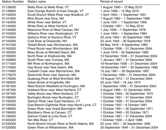
Table 1. List of streamgauges used to estimate unregulated, daily streamflow at ungauged locations in the Connecticut River Basin.

Station Number Station name Period of record

01073000 Oyster River near Durham, NH 15 December 1934 – 31 December 2004 01082000 Contocook River at Peterborough, NH 7 July 1945 – 30 September 1977 01084500 Beard Brook near Hillsboro, NH 1 October 1945 – 30 September 1970 01085800 West Branch Warner River near Bradford, NH 22 May 1962 – 30 September 2004 01086000 Warner River at Davisville, NH 1 October 1939 – 30 September 1978 01089000 Soucook River near Concord, NH 1 October 1951 – 30 September 1987 01091000 South Branch Piscataquog River near Goffstown, NH 27 July 1940 – 30 September 1978 01093800 Stony Brook tributary near Temple, NH 1 May 1963 – 30 September 2004 01096000 Squannacook River near West Groton, MA 1 October 1949 – 31 December 2004 01097300 Nashoba Brook near Acton, MA 26 July 1963 – 31 December 2004 01105600 Old Swamp River near South Weymouth, MA 20 May 1966 – 24 July 2006 01105730 Indian Head River at Hanover, MA 8 July 1966 – 24 July 2006

01106000 Adamsville Brook at Adamsville, RI 1 October 1940 – 30 September 1978 01108000 Taunton River near Bridgewater, MA 1 October 1929 – 23 April 1976 01109000 Wading River near Norton, MA 1 June 1925 – 31 December 2004 01111300 Nipmuc River near Harrisville, RI 1 March 1964 – 30 September 1991 01111500 Branch Riverb at Forestdale, RI 24 January 1940 – 31 December 2004 01117500 Pawcatuck River at Wood River Junction, RI 7 December 1940 – 31 December 2004 01118000 Wood River Hope Valley, RI 12 March 1941 – 31 December 2004 01118300 Pendleton Hill Brook near Clarks Falls, CT 1 October 1958 – 31 December 2004 01118500 Pawtucket River at Westerly, RI 27 November 1940 – 31 December 2004 01120000 Hop Brook near Columbia, CT 1 October 1932 – 6 October 1971 01121000 Mount Hope River near Warrenville, CT 1 October 1940 – 31 December 2004 01123000 Little River near Hanover, CT 1 October 1951 – 31 December 2004 01127880 Big Brook Near Pittsburg Nh 1 December 1963 – 1 January 1984 01133000 East Branch Passumpsic River near East Haven, VT 1 October 1948 – 1 September 1979 01133500 Passumpsic River near St. Johnsbury, VT 1 May 1909 – 1 July 1919

(17)

GMDD

5, 2503–2526, 2012

Tables Figures

◭ ◮

Back Close

Full Screen / Esc

Discussion

P

a

per

|

Dis

cussion

P

a

per

|

Discussion

P

a

per

|

Discussio

n

P

a

per

|

Table 1.Continued

Station Number Station name Period of record

01139000 Wells River at Wells River, VT 1 August 1940 – 12 May 2010 01139800 East Orange Branch at East Orange, VT 1 June 1958 – 12 May 2010 01140000 South Branch Waits River near Bradford, VT 1 April 1940 – 1 September 1951 01141800 Mink Brook near Etna, NH 1 August 1962 – 1 September 1998 01142000 White River near Bethel, VT 1 June 1931 – 1 September 1955 01144000 White River at West Hartford, VT 1 October 1951 – 12 May 2010 01145000 Mascoma River at West Canaan, NH 1 July 1939 – 1 September 1978 01153500 Williams River near Rockingham, VT 1 June 1940 – 1 September 1984 01154000 Saxtons River at Saxtons River, VT 20 June 1940 – 30 September 1982 01155000 Cold River at Drewsville, NH 23 June 1940 – 30 September 1978 01161500 Tarbell Brook near Winchendon, MA 29 May 1916 – 6 September 1983 01162500 Priest Brook near Winchendeon, MA 1 October 1936 – 31 December 2004 01165500 Moss Brook at Wendell Depot, MA 1 June 1916 – 30 September 1982 01169000 North River at Shattuckville, MA 13 December 1939 – 31 December 2004 01169900 South River near Conway, MA 1 January 1967 – 31 December 2004 01171500 Mill River at Northampton, MA 18 November 1938 – 31 December 2004 01174000 Hop Brook near New Salem, MA 19 November 1947 – 30 September 1982 01174900 Cadwell Creek near Belchertown, MA 13 July 1961 – 30 September 1997 01175670 Sevenmile River near Spencer, MA 1 December 1960 – 31 December 2004 01176000 Quaboag River at West Brimfield, MA 19 August 1912 – 31 December 2004 01180000 Sykes Brook at Knightville, MA 20 June 1945 – 18 July 1974

(18)

GMDD

5, 2503–2526, 2012

Tables Figures

◭ ◮

Back Close

Full Screen / Esc

Discussion

P

a

per

|

Dis

cussion

P

a

per

|

Discussion

P

a

per

|

Discussio

n

P

a

per

|

Table 2.Number of streamgauges, goodness of fit values, explanatory variables, and estimated regression parameters for streamflows estimated from catchment characteristics. (%RMSE,

Percent root-mean square error;∗∗, characteristic not included in regression equation;†, Bias

correction factor computed from Duan (1983); NSE, Nash-Sutcliffe efficiency value).

General regression information Characteristics in the regression equation and coefficient value

Exceedence probability

Number of stream-gauges used to develop regression equation

%RMSE NSE Constant

term

Drainage area

Average annual precip-itation.

Percent of basin that is underlain by sand and gravel deposits

Y-location of the basin centroid

X-location of the basin centroid

Bias correla-tion factor†

0.02 51 1.49 0.99 −26.5758 0.9590 2.3262 ∗∗ _1.4462 ∗∗ _1.0103

0.05 51 0.62 1.00 −19.3148 0.9775 1.7521 ∗∗ _1.0457 ∗∗ _1.0023

0.1 51 0.73 0.99 −2.1224 0.9982 0.9106 ∗∗ ∗∗ ∗∗ _1.0015

0.15 51 0.60 1.00 −2.9777 1.0050 1.0589 ∗∗ ∗∗ ∗∗ _0.9972

0.2 51 0.86 0.99 −3.6935 1.0037 1.1920 ∗∗ ∗∗ ∗∗ _0.9957

0.25 51 1.32 0.98 −4.6684 1.0110 1.3890 ∗∗ ∗∗ ∗∗ _0.9950

0.3 51 1.86 0.98 −5.5394 1.0137 1.5688 ∗∗ ∗∗ ∗∗ _0.9950

0.4 51 3.00 0.96 −6.7591 1.0206 1.8000 ∗∗ ∗∗ ∗∗ _0.9960

0.5 51 3.86 0.95 −7.6803 1.0269 1.9577 ∗∗ ∗∗ ∗∗ _0.9982

0.6 50 4.40 0.96 −8.3466 1.0184 2.0123 0.0804 ∗∗ ∗∗ _1.0184

0.7 50 6.61 0.94 −8.4500 1.0480 1.9072 0.0949 ∗∗ ∗∗ _1.0278

0.75 50 9.24 0.93 −8.7450 1.0655 1.9073 0.1040 ∗∗ ∗∗ _1.0243

0.8 50 13.58 0.92 −9.1085 1.0951 1.9008 0.1251 ∗∗ ∗∗ _1.0379

(19)

GMDD

5, 2503–2526, 2012

Tables Figures

◭ ◮

Back Close

Full Screen / Esc

Discussion

P

a

per

|

Dis

cussion

P

a

per

|

Discussion

P

a

per

|

Discussio

n

P

a

per

|

Table 3.Number of streamgauges, goodness of fit values, explanatory variables, and estimated regression parameters for streamflows estimated from other streamflow quantiles. (%RMSE,

Percent root-mean square error;†, Bias correction factor computed from Duan (1983); NSE,

Nash-Sutcliffe efficiency value).

General regression information Characteristics in the regression equation and coefficient value Exceedence

probability

Number of streamgauges used to develop regression equation

%RMSE NSE Constant term

Coefficient on explana-tory variable

Explanatory variable

Bias correla-tion factor†

0.9 50 32.36 0.89 −0.4112 1.0511 Streamflow at the 0.85 exceedence probability

1.0004

0.9986

1.0103

1.0000

0.999938 34 825.08 −1.30 −1.6658 1.2826 Streamflow at the 0.99 exceedence probaility

(20)

GMDD

5, 2503–2526, 2012

Tables Figures

◭ ◮

Back Close

Full Screen / Esc

Discussion

P

a

per

|

Dis

cussion

P

a

per

|

Discussion

P

a

per

|

Discussio

n

P

a

per

|

Table 4.Variogram model parameters and root-mean-square error value resulting from a leave-one-out cross validation of the variogram models.

Station Number

Variance parameter Range parameter Root-mean-square error

(21)

GMDD

5, 2503–2526, 2012

Tables Figures

◭ ◮

Back Close

Full Screen / Esc

Discussion

P

a

per

|

Dis

cussion

P

a

per

|

Discussion

P

a

per

|

Discussio

n

P

a

per

|

COMPUTE CHARACTERISTICS

AT UNGAUGED CATCHMENT

TIME

S

T

R

E

A

M

F

L

O

W

SELECT REFERENCE STREAMGAGE USING

LOCATION COORDINATES AND MAP CORRELATION

ESTIMATE THE FLOW-DURATION CURVE

AT THE UNGAUGED CATCHMENT

COMPUTE THE FLOW-DURATION CURVE

AT THE GAUGED CATCHMENT OBTAIN THE STREAMFLOW

AT THE GAUGED CATCHMENT

ESTIMATE THE STREAMFLOW AT THE UNGAUGED CATCHMENT SELECT THE UNGAUGED

STREAM LOCATION AND DELINEATE CATCHMENT AREA

EXPLANATION

Action executed by the StreamStats tool

TIME

S

T

R

E

A

M

F

L

O

W

S

T

R

E

A

M

F

L

O

W

EXCEEDANCE PROBABILITY 0 0.10.20.3 0.40.5 0.6 0.70.80.9 1

S

T

R

E

A

M

F

L

O

W

EXCEEDANCE PROBABILITY 0 0.10.20.3 0.40.5 0.6 0.70.80.9 1

(22)

GMDD

5, 2503–2526, 2012

Tables Figures

◭ ◮

Back Close

Full Screen / Esc

Discussion

P

a

per

|

Dis

cussion

P

a

per

|

Discussion

P

a

per

|

Discussio

n

P

a

per

|

Streamflows interpolatied between selected qunatiles to obtain continuous curve

NATURAL LOG OF S

T

R

E

A

M

F

L

O

W

EXCEEDANCE PROBABILITY

0 0.1 0.2 0.3 0.4 0.5 0.6 0.7 0.8 0.9 1

Streamflows estimated by the drainage-area ratio:

Flow quantiles greater than 0.01

Flow quantiles between 0.01 and 0.85

Flow quantiles less than 0.85 Qungaged(p) =Areaungaged_Areagaged Qgaged(p)

Streamflows estimated by regression of selected qunatiles against

characteristics.

Streamflows estimated recusively by regression against streamflows at other selected

quantiles. 6

3

0

LOG STREAMFLOW AT THE

85-PERCENT EXCEEDANCE PROBABILITY

99.9938-PERCENT EXCEEDANCE PROBABILITY

(THE LOWEST FLOW IN A 44-YEAR DAILY FLOW RECORD)

3

0

-3

4

0

-4

5

0

-5 4

2 0

5

0

-5 5

2.5 0

3 0

4 0 -4

5 0 -5

(23)

GMDD

5, 2503–2526, 2012

Tables Figures

◭ ◮

Back Close

Full Screen / Esc

Discussion

P

a

per

|

Dis

cussion

P

a

per

|

Discussion

P

a

per

|

Discussio

n

P

a

per

|

Fig. 3.Screen captures showing the decision-support tool used to estimate daily, unregulated time series. The program delineates a catchment for the ungauged location selected by the user

(A)and summarizes the catchment characteristics(B). The user then inputs these

character-istics into a spreadsheet program(C–E)that generates the daily, period of record flow-duration

(24)

GMDD

5, 2503–2526, 2012

Title Page Abstract Introduction Conclusions References Tables Figures ◭ ◮ ◭ ◮ Back Close

Full Screen / Esc

Printer-friendly Version Interactive Discussion Discussion P a per | Dis cussion P a per | Discussion P a per | Discussio n P a per |

0 43,750 87,500meters 01333000 01332000 01200000 01193500 01188000 01187300 01181000 01176000 01171500 01169000 01165500 01162500 01154000 01153500 01144000 01139800 01139000 01137500 01135000 01134500 01123000 01121000 01118500 01118300 01117500 01111500 01109000 01096000 01073000 01161500 01118000 EXPLANATION

Efficiency value at the streamgage

State boundary Connecticut River Basin

> 0.90 Between 0.85 and 0.90 Between 0.80 and 0.85 Between 0.75 and 0.80

< 0.70 (minimum value is 0.69) Between 0.70 and 0.75 0 500 1000 1500 2000 2500 10/1/1960 1/ 1/ 19 61 4/1 /19 61 7/ 1/ 19 61 10/1/1961 1/ 1/ 19 62 4/1 /19 62 7/ 1/ 19 62 Estimated streamflow Observed streamflow Estimated streamflow Observed streamflow Estimated streamflow Observed streamflow 0 500 1000 1500 2000 2500 3000 3500

10/1/1960 1/1/1961 4/1/1961 7/1/1961 10/1/1961 1/1/1962 4/1/1962 7/1/1962

0 25 50 75 100 125 10 /1 /1 96 0

1/1/1961 4/1/1961 7/1/1961 10/1

/1

96

1

1/1/1962 4/1/1962 7/1/1962

STREAMFLOW

, IN CUBIC FEET

PER SECOND

STREAMFLOW

, IN CUBIC FEET

PER SECOND

STREAMFLOW

, IN CUBIC FEET

PER SECOND 01188000 01153500 01137500 1.0 0.9 0.8 0.7 0.6 0.5 0.4 0.3 0.2 0.1 0.0 NASH-SUTCLIFFE EFFICIENCY EXPLANATION Median 25th percentile 75th percentile Upper limit (75th percentile + 1.5 * (75th percentile - 25th percentile))

Lower limit (25th percentile + 1.5 * (75th percentile - 25th percentile)) Values above the upper limit or below the lower limit

COMPUTED FROM OBSERVED AND

ESTIMATED STREAMFLOWS

COMPUTED FROM THE NATURAL LOGS OF THE OBSERVED AND ESTIMATED STREAMFLOWS A B C D E

Fig. 4.Range of efficiency values computed between the observed and estimated streamflows

at the 31 validation streamgauges(A), spatial distribution of efficiency values resulting from

log-transformed observed and estimated daily streamflow at 31 validation streamgauges(B)and

selected hydrographs of observed and estimated streamflow for the period from 1 October 1960