Evaluation of gene selection metrics for tumor cell classification

Evaluation of gene selection metrics for tumor cell classification

Katti Faceli

, André C.P.L.F. de Carvalho

and Wilson A. Silva Jr

1

Universidade de São Paulo, Instituto de Ciências Matemáticas e de Computação, São Carlos, SP, Brazil.

2

_{Faculdade de Medicina de Ribeirão Preto, Departamento de Genética, Centro de Terapia Celular,}

Laboratório de Genética Molecular e Bioinformática, Ribeirão Preto, SP, Brazil.

Abstract

Gene expression profiles contain the expression level of thousands of genes. Depending on the issue under investigation, this large amount of data makes analysis impractical. Thus, it is important to select subsets of relevant genes to work with. This paper investigates different metrics for gene selection. The metrics are evaluated based on their ability in selecting genes whose expression profile provides information to distinguish between tumor and normal tissues. This evaluation is made by constructing classifiers using the genes selected by each metric and then comparing the performance of these classifiers. The performance of the classifiers is evaluated using the error rate in the classification of new tissues. As the dataset has few tissue samples, the leave-one-out methodology was employed to guarantee more reliable results. The classifiers are generated using different machine learning algorithms. Support Vector Machines (SVMs) and the C4.5 algorithm are employed. The experiments are conduced employing SAGE data obtained from the NCBI web site. There are few analysis involving SAGE data in the literature. It was found that the best metric for the data and algorithms employed is the metric logistic.

Key words:gene selection, machine learning, gene expression, sage.

Received: August 15, 2003; Accepted: August 20, 2004.

Introduction

This investigation was developed as part of the FAPESP/LIRC Clinical Genomics Project, that involves several Brazilian research groups. The main goal of this project is to study gene expression in neoplasias and de-velop approaches that may be relevant to clinical applica-tions, either to identify disease markers or to define profiles related to clinical evolution or outcome. This paper investi-gates metrics to support the biologists in the selection of genes that could be related to the occurrence of some neoplasias, based on their expression profiles.

Today, there are several methods to monitor the ex-pression level of a large amount of genes simultaneously. These large-scale gene expression analysis methods can be summarized in two main groups: the tag counting methods (SAGE, MPSS) and the hybridization-based methods (cDNA, oligonucleotide microarray). There are also sev-eral analyses that can be carried out with gene expression data, involving pairwise or multiple condition analysis (Claverie, 1999).

In spite of the method employed to acquire the gene expression data, their analysis involves several aspects that have been addressed in the literature (Brazma and Vilo, 2000; Dopazoet al., 2001). One of these aspects is gene se-lection. Gene expression profiles present the expression level of thousands of genes. Depending on the issue under investigation, this large amount of data makes the analysis impractical. Besides, and more importantly, large changes in a particular phenotype can be due to changes in the ex-pression of a small subset of its genes. Thus, it is important to select subsets of relevant genes to work with. In sum-mary, the interest in a small set of genes can be motivated by financial, personal workload or experimental reasons. Gene selection gives the biologists a small set of genes to make more specific, complex and usually expensive inves-tigations.

There are several methods reported in the literature that have been applied to gene selection (Slonim et al., 2000; Golubet al., 1999; Zhang and Wong, 2001; Ben-Dor

et al., 2000; Ben-Dor et al., 2002; Jaeger et al., 2003; Claverie, 1999). Most of them are feature-ranking niques, frequently called scores. In this work, these tech-niques will be called metrics. Some of these metrics measure the similarity between the gene expression vector and the class vector (correlation metrics). Other metrics

Send correspondence to André C.P.L.F. de Carvalho. Universi-dade de São Paulo, Instituto de Ciências Matemáticas e de Com-putação, Departamento de Ciências de Computação e Estatística, Avenida Trabalhador Sancarlense 400, Centro, Caixa Postal 668, 13566-590 São Carlos, SP, Brazil. Email: andre@icmc.usp.br.

evaluate the difference between the same vectors (distance metrics). Additionally, there are methods described in the literature that are based on genetic algorithms (Liuet al., 2001), feature selection (Inza et al., 2002) and Support Vector Machines (Guyonet al., 2002; Zhang and Wong, 2001).

Many researchers use filtering rules based on fold dif-ference criteria to select subsets of genes. For example, Schenaet al.(1996) selected only those genes for which the ratios between the expression intensities of the two condi-tions being investigated were higher than twofold (Dopazo

et al., 2001). However, the application of a simple rule, fold-based, can lead to a high number of false positives (Claverie, 1999). Slonimet al.(2000) employed a number of metrics to rank oligonucleotide microarray data, such as the Pearson correlation coefficient and Euclidean distance, and proposed a correlation metric that emphasizes the “sig-nal-to noise” ratio in using the gene as a predictor, called here Golub’s score. Ben-Doret al.(2000) examined several scoring methods for mining relevant genes. They employed the TNoM and INFO scores, a score based on Logistic regression and the Golub’s score. For their analysis, they employed two datasets obtained from oligonucleotide microarrays and one data set obtained from cDNA micro-arrays.

In the present paper, the authors investigate six met-rics commonly used to select genes from microarray data, to select genes based on their expression level obtained with the SAGE technique. The metrics employed here rep-resent a combination of those employed by Schenaet al.

(1996), Slonimet al.(2000) and Ben-Doret al.(2000). The metrics employed in this paper are evaluated according to their ability in selecting predictive genes. This evaluation is made by constructing classifiers using as attributes the genes selected by each metric and then comparing the per-formance of these classifiers. The classifiers are generated using Support Vector Machines (SVMs) (Cristianini and Shawe-Taylor, 2000) and C4.5 (Quinlan, 1993).

In contrast to this paper, the papers found in the litera-ture that describe metrics for gene selection usually do not compare a large number of metrics and apply the metrics to microarray data. There are few analyses involving SAGE

data described in the literature and none with all the metrics evaluated here. The comparison of all these metrics and their application to SAGE data are the main contributions of this work. The comparison of two well-known learning algorithms for the analysis of the metrics using SAGE data can also be considered a contribution.

Material and Methods

Data set

The data set employed in the paper was obtained from the Cancer Genome Anatomy Project - CGAP1. The au-thors selected 40 libraries containing expression profiles from normal and cancerous brain tissues. Each library rep-resents a different tissue or condition and contains the tag, the frequency of the tag, the associated unigene number and an annotation about the gene. In order to create the data set used in the classification experiments, the libraries were combined in a unique file, with the rows representing a gene (each row corresponds to a tag-unigene combination) and the columns representing the tissues or conditions. This file contains seven columns of normal tissues and 33 col-umns of cancerous tissues. When a tag is not found in a li-brary, its frequency is set to 0.

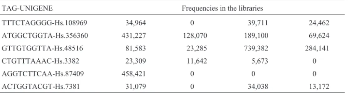
The file generated contains 285,723 tags representing the genes. In this file, a normalization operation was ap-plied to the frequencies, to adjust for libraries to have the same total number of tags. All libraries were adjusted to have a total of 200,000 tags (new frequency = original fre-quency * 200,000 / total number of tags). Next, a filter was applied to the data to remove tags that contain errors and imprecisions due to SAGE. The genes with expression level (frequency) smaller than 24 in all libraries were re-moved from the file. This filtering kept only 7,888 genes. Table 1 shows a portion of the file generated.

Gene selection

The choice of the approach for gene selection de-pends very much on the properties the researcher wants to measure (Dopazoet al., 2001). Most of these approaches described in the literature are feature ranking techniques, also called scores or metrics. In this work, these techniques

Table 1- Portion of the main dataset.

TAG-UNIGENE Frequencies in the libraries

TTTCTAGGGG-Hs.108969 34,964 0 39,711 24,462

ATGGCTGGTA-Hs.356360 431,227 128,070 189,100 69,624

GTTGTGGTTA-Hs.48516 81,583 23,285 739,382 284,141

CTGTTTAAAC-Hs.3382 23,309 11,642 5,673 0

AGGTCTTCAA-Hs.87409 458,421 0 0 0

ACTGGTACGT-Hs.7381 31,079 0 34,038 13,172

will be called metrics. Some of these metrics measure the similarity (correlation metrics) and others measure the dif-ference (distance metrics) between the gene expression vector and the class vector.

The metrics or scores can be divided into parametric and nonparametric scores. The parametric scores make as-sumptions about the form of the statistical distribution of the scores within each group, while the nonparametric scores do not make such assumptions, and are more robust (Ben-Doret al., 2002).

The nonparametric metrics generally specify a hy-pothesis in terms of population distributions, rather than parameters like means and standard deviations. These metrics are almost as capable of detecting differences among populations as the parametric scores when normal-ity and other assumptions need to be satisfied. Nonparametric scores may be, and often are, more power-ful in detecting population differences when these as-sumptions are not satisfied.

In the present work, the authors compare the fold change criteria (FC), the difference (Diff), the Golub’s, TNoM and INFO scores, a score based in Logistic regres-sion (Logistic), the Euclidean distance (Euclidean) and the Pearson correlation coefficient (Pearson). All these metrics are detailed in the next subsection.

For the analysis performed, the authors decided to evaluate subsets of 100, 10 and 4 genes. The gene selection was carried out in the following way. First, all metrics were calculated for each gene of the SAGE data set previously described. Next, the data were sorted according to the rank-ing provided by each metric. Subsets with the 100, 10 and 4 genes with the best values for each metric were then se-lected (for each metric, three data sets were produced - with 100, 10 and 4 genes). The best value for the Euclidean dis-tance, TNoM, INFO and Logistic metrics means the lowest values. For the FC, Diff, Golub and Pearson metrics, the highest positive values were chosen as representing the most hyper-expressed genes and the smallest negative val-ues were chosen as representing the most hypo-expressed genes in tumor tissues. Half of the genes selected were hy-per-expressed and the other half were hypo-expressed genes. The genes selected generated the data sets employed later in the training of the machine learning algorithms. The three data sets generated for each metric are composed of 40 tissues (conditions) as samples and 100, 10 and 4 genes as attributes or features. Table 2 contains a summary de-scription of these datasets.

The selection process resulted in 24 data sets (8 met-rics x 3 number of genes selected). With these data sets, the authors generated SVM and C4.5 classifiers. The metrics were evaluated according to the performance of the classi-fiers. The performance for each dataset in the classification of new tissues was obtained by performing leave-one-out crossvalidation (Mitchell, 1997). A good metric is one that selects the best set of genes to distinguish the classes (nor-mal and tumor tissues), and a good class distinction is de-tected by low error rates in the classification of new tissues.

The SVMs were trained with linear kernels. Only this kernel was employed because results of previous similar works show the worst results were attained with the Gaussi-an Gaussi-and polinomial kernels.

Metrics

The metrics FC and Diff refer to the comparison of two conditions. The dataset analyzed has multiple condi-tions for each type of tissue (several normal and several tu-mor tissue libraries). For these metrics, the authors considered the libraries of each type of tissue as a pool. The expression level of each gene in a pool is the mean of the expression levels of the gene in each library.

Letmbe the number of genes andnbe the number of samples or tissues. Each gene in the dataset, or gene expres-sion matrix, can be represented by a gene expresexpres-sion vector

g∈Rn. This work centers the discussion in the case where there are two groups of conditions to be compared. In this case, there are two classes in which the data samples can be separated. These classes will be represented here as -1, or

neg(for example, a control condition, such as normal tis-sues) and +1, orpos(for example, the experimental condi-tion being investigated, such as cancerous tissues). A class vectorc∈{-1, 1}nrepresents the two-class distinction pre-sented in the data. The within-class mean,µx, is the mean of

the expression levels of the samples in classxfor a particu-lar gene. The within-class standard deviation, σx, is the standard deviation of the expression levels of the samples in the classxfor a particular gene.

To calculate the TNoM, INFO and Logistic metrics, the software scoreGenes2was employed. Next, each metric used is briefly described.

• Fold change

This metric involves the calculation of a ratio relating the expression level of a gene under two experimental con-ditions. These conditions are, usually, a control and an

un-Table 2- Description of the data sets characteristics.

Number of samples Number of features (genes) Percentage of tissues Majority error Missing values

40 100, 10 and 4 17.5% normal

82.5% tumor

17.5% no

der investigation condition, such as normal and tumor tissue samples. An arbitrary ratio (usually 2-fold) is then se-lected as being significant. The cDNA microarray data are already represented as ratio, because most of cDNA microarrays involves two-color fluorescence competitive assays. But when analyzing SAGE or oligonucleotide microarrays the ratio (or FC) has to be calculated.

When only two experiments are compared, the ratio can be calculated directly. However, in some cases, there are several experiments for each of the two classes of inter-est. In these cases, the mean of the expression values can be calculated for each class and the ratio can be taken from these values. The authors are employing the last case, so the formulas using the mean as the expression values for each class will be shown.

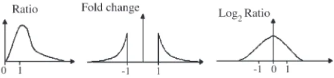
The metric involving the ratio can be expressed in three different ways: the ratio itself, the fold change way and the log of the ratio. Their formulas can be observed in the Equations 1, 2 and 3, respectively.

R pos

neg

=µ

µ (1)

FC

R, R 1

1-1 R R 1

=

≥

< 

 

 ,

(2)

LR=log R2 (3)

The shortcoming of R is that the hyper-expression, or induction, and hypo-expression, or repression, are repre-sented by values of different magnitude. For example, a two-fold induction will have more weight than a one-half repression in any comparison. (Dopazoet al., 2001). The FC and LR metrics overcome this problem. In these met-rics, the induction and repression have the same magnitude. The graphics of the three kinds of ratio can be observed in Figure 1. Equation 3 represents alog2transformation, but

other logarithms can be applied. In this case, a twofold in-duction is indicated by the value 1 and a one-half repression by the value -1.

• Difference

This metric is the difference between the mean of the expression values of the tumor samples and the mean of the expression values of the normal samples, as shown by Equation 4.

Diff=µpos −µneg (4)

• Euclidean distance

This metric measures the absolute distance between two points in space. These points can be two profiles, or, as in this case, one profile and the class vector. Usually, this metric does not require the data to be normalized, and con-siders profiles of genes with the same magnitude to be simi-lar. However, sometimes, one is looking for genes expressed at different levels, but with the same overall

ex-pression. For this purpose, the data should be re-scaled and normalized. In the experiments described in this work, when a gene expression profile is being compared to the class vector, the expression values need to be re-scaled to be comparable to the class vector. The formula of the Eu-clidean distance is shown in Equation 5. In this work, g_norm is the gene expression vector re-scaled to the inter-val [-1, 1] and ciis the class vector where -1 represents

tu-mor tissue and 1 represents normal tissue.

Euclidean 1

n (g_ norm -c )i i

2

i=1 n

=

∑

• Pearson correlation coefficient

The formula of Pearson correlation coefficient can be seen in Equation 6, where g_norm is the gene expression vector normalized to have zero mean and variance 1 and ci

is the class vector, where -1 represents tumor tissue and 1 represents normal tissue.

Pearson 1

n i=1g_ norm ci i n

=

∑

This metric usually does not need any transformation to be applied to the data. But, in this case, the gene expres-sion vector is normalized because it is being compared to the class vector, employing a simplified equation. The val-ues resulting from this metric lie between -1, meaning a negative correlation, and 1, meaning a positive correlation. Thus, a value of 0 indicates no correlation between the gene and the class vector.

• Golub

This is a correlation metric proposed by Golubet al.

(Golubet al., 1999; Slonimet al., 2000). Its formula can be seen in Equation 7. It measures relative class separation. This metric reflects the difference between the classes rela-tive to the standard deviation within the classes. Large val-ues ofGolubindicate a strong correlation between gene expression and class distinction. The sign of Golub corre-sponds togbeing more highly expressed in the classposor

neg. The values of this metric are not confined to the range [-1,1].

Golub

+

pos neg

pos neg

=µ −µ

σ σ (7)

Referred to by Ben-Doret al.(2000) as a Gaussian separation score, the Golub metric attempts to, using a

Gaussian approximation, measure to what extent thepos

andnegclasses are separated. Intuitively, the separation be-tween two groups of expression values is proportional to the distance between their mean. This distance has to be normalized by the standard deviation of the groups. A large standard deviation indicates points in the group far away from the mean value and thus the separation would not be strong.

• TNoM score

The TNoM (Threshold Number of Misclassification) score (Ben-Doret al., 2000; Ben-Doret al., 2002) calcu-lates a minimal error decision boundary and counts the number of misclassifications carried out with this bound-ary.

This score is based on the idea that a genegis relevant to the tissue partition if it is over-expressed in one of the classes. This can be formalized by considering howg’s ex-pression levels in the classposrelates to its expression lev-els in the class neg. Let t be a vector of the ordered expression levels ofg(t1is the minimum andtnis the

maxi-mum expression level ofg). A rank vector,v, ofgis defined as a vector of lengthnwhereviis the label associated withti.

Ifgis under-expressed in the classpos, then theposentries ofvare concentrated in the left hand side of the vector and thenegentries are concentrated at the right hand side. Simi-larly for the opposite situation. Thus, the relevance ofg in-creases as the homogeneity within the left hand side and within the right hand side ofvincreases. On the other hand, ifgis not informative with respect to the given labeling, the

posandneginvare interleaved.

The TNoM score comes from a natural way of defining the homogeneity on the two sides and then combining them into one score. The score ofvcorresponds to the maximal combined homogeneity over all possible ways to breakvin two parts, a prefixx, consisting of mostlyposand a suffixy, consisting of mostlyneg, or vice versa. The TNoM score ofv

corresponds to the partition that best dividesvinto a homo-geneous prefixxand a homogeneous suffixy.

The MinCardinality (MC) of apos-negvectorxis the cardinality of the minority symbol inx, as can be seen in Equation 8, where#s(x)is the number of times a symbols

appears in the vectorx. The TNoM score can be seen in the Equation 9.

MC = min(# neg(x), #pos(x)) (8)

TNoM (v)= min

:

x y v= (MC(x), MC(y)) (9)

• INFO score

This score, similarly to TNoM, measures the level of homogeneity of the partitions of the rank vector ofg. How-ever, it does not count the number of misclassified samples. Instead, it uses the notion of conditional entropy. Letwbe a vector composed ofposandnegsamples, and letpdenote

the fraction of theposentries inw. The entropy ofwis de-fined according to Equation 10.

H(w) = -plogp- (1 -p) log (1 -p) (10)

The entropy measures the information in the vectorw. This quantity is non-negative, and equal to 0 if and only if

p= 0 orp= 1, that is, if w is homogeneous. The maximal value of H(w) is 1 when w is composed of an equal number ofposandneglabels.

The INFO score ofv is defined to be the minimal weighted sum of the entropies of a prefix-suffix division, as can be seen in Equation 11, where.is the length of the vector. This is the conditional entropy of the rank vector given the partition of the samples in two groups (x and y).

INFO(v) = min

:

x y v= +

  

  

x v H(x)

y

v H(y) (11)

• Logistic

This metric is based on Logistic regression, as de-scribed by Ben-Doret al.(2000). The main idea of this met-ric is to have the probability of both labels close to 0.5, when the expression values are close to the decision thresh-old and confident for extreme expression values. The con-ditional probability is either 0 or 1. Such concon-ditional probabilities can be represented by the logistic family:

l_{log it}(pos x:a, b)=logit(ax b)+ (12)

where logit(z) is the logistic function in Equation 13.

log it(z) 1 1 e z =

+ − (13)

To score a gene using this metric, it is necessary to find the parametersaandbthat minimize the logloss func-tion. This can be carried out by gradient based non-linear optimization.

Learning algorithms employed

The algorithms employed in this work to classify the tissue samples produced by SAGE technique are Support Vector Machines (SVMs) (Cristianini and Shawe-Taylor, 2000) and the C4.5 algorithm (Quinlan, 1993).

ob-tained by projecting it from the input space to the feature space and classifying it based on its position relative to the separating hyperplane.

C4.5 is a learning algorithm that generates models in the form of decision trees. It builds a decision tree from training data by applying a divide-and-conquer strategy and employing a greedy approach that uses a gain ratio as its guide. It chooses an attribute for the root of the tree, di-vides the training instances into subsets corresponding to the values of the attribute and test the gain ratio on this at-tribute. This process is repeated for all input attributes of the training patterns. C4.5 chooses the attribute that gains the most information to be at the root of the tree. The algo-rithm is applied recursively to form sub-trees, terminating when a given subset contains instances of only one class (Quinlan, 1993).

Results

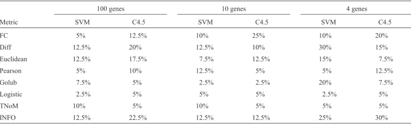
Table 3 presents the error rates obtained in the evalua-tion of the classifiers generated with each metric and num-ber of genes selected. From this table, it can be observed that most of the lowest errors were achieved with the Logis-tic metric (with 100 and 4 genes). In these cases, the lowest errors were 2.5% for SVM and 5% for C4.5. For 10 genes, the metric Golub presented the lowest error (2.5%), for both SVM and C4.5. An error of 2.5% means that only one tissue was wrongly classified. Although Golub has sented the best results with 10 genes, Logistic also pre-sented low error rate (5%). In most of the cases, the results obtained with C4.5 were worse than those obtained with SVM.

For the cases of 100 and 4 genes, other metrics pre-sented the same level of error of Logistic as the algorithm C4.5 (100 genes: Golub and TNoM, 4 genes: TNoM). In most of the cases, the TNoM metric showed an error of 5% (2 samples wrongly classified), and in the other cases an er-ror of 10%.

Discussion

The analysis performed in this work encompasses the metrics employed in the works of Schena et al. (1996), Slonimet al.(2000) and Ben-Doret al.(2000). This work compares the metrics in the context of SAGE data, while these authors employed them for microarray data.

Each of these metrics has its shortcomings. The choice of the best metric for an analysis should take into ac-count the data to be analyzed.

The selection of an arbitrary threshold for the fold change metric results in low specificity and low sensitivity. The low specificity is related to the false positives, particu-larly with low-abundance transcripts or when a data set is derived from a divergent comparison. The low sensitivity is related to the false negatives, particularly with high-abundance transcripts or when a data set is derived from a closely linked comparison. This metric has several short-comings and it is now accepted that its use should be dis-continued (Murphy, 2002). It also should be noted that this kind of metric removes all information about the absolute gene expression levels.

The Golub metric works well for data normally dis-tributed in each class.

The TNoM score provides partial information about the quality of the predictions made by the best rules. For ex-ample, there is no distinction between a rule that makesk

one-sided errors (for example, all the errors are samples of classpospredicted asneg) and a rule that makesk/2errors of the second kind. This distinction is important, since the performance of a rule, such as the one initially described, is very poor for one of the classes. The INFO score makes such distinctions finer.

In the present work, the metrics are compared accord-ing to the error rate of the classifiers generated with the genes selected by the metrics.

As expected, the simplest metrics, FC and Diff, pre-sented high error rates. Although these high errors did not occur in all cases, these results suggest that relying only on these metrics to select genes is not appropriate. Such a

con-Table 3- Summary of the errors.

100 genes 10 genes 4 genes

Metric SVM C4.5 SVM C4.5 SVM C4.5

FC 5% 12.5% 10% 25% 10% 20%

Diff 12.5% 20% 12.5% 10% 30% 15%

Euclidean 12.5% 17.5% 7.5% 12.5% 15% 7.5%

Pearson 5% 10% 12.5% 5% 5% 12.5%

Golub 7.5% 5% 2.5% 2.5% 20% 7.5%

Logistic 2.5% 5% 5% 5% 2.5% 5%

TNoM 10% 5% 10% 5% 5% 5%

clusion just confirms the characteristics of the metrics pre-sented.

In a few cases, the classifiers generated presented an error superior to the majority error. These classifiers did not learn the class separation, and were equivalent to a classi-fier that just assigns all samples to the tumor class. Metrics that produced such classifiers in at least one case were the FC, Diff, Euclidean, Golub and INFO metrics.

The metric Golub showed unstable behavior. It pre-sented the best result in some cases, the worst result in an-other and an intermediate result in an-other cases.

The most stable metrics were the Logistic and TNoM metrics. These metrics presented the same error for the C4.5, but the Logistic metric was more accurate when SVM was employed.

Looking at the results obtained, it is not possible to es-tablish the influence of the number of genes selected in the classification.

Conclusion

This paper investigated six metrics commonly used to select genes from microarray data, to select genes based on their expression level obtained with the SAGE technique. The metrics were evaluated based on their ability in select-ing predictive genes. This evaluation was made by con-structing classifiers using the genes selected and comparing their performance. The classifiers were generated using the SVM and C4.5 techniques.

The best classifiers were generated with the metrics Logistic in most of the cases. The lowest error rates, 2.5%, were achieved with at least one classifier generated with SVM for each number of genes and with one classifier gen-erated with C4.5 for the case of 10 genes.

The comparison of all these metrics and their applica-tion to SAGE data are the main contribuapplica-tions of this work.

There are several other metrics for gene selection de-scribed in the literature. It would be interesting to integrate a few more common metrics in the present analysis as a fu-ture work. Another fufu-ture step is the application of the same evaluation described in this paper to other data sets. It is im-portant to evaluate the behavior of the metrics for micro-array data too.

Acknowledgments

This research was supported in part by the Brazilian Research Councils FAPESP and CNPq.

References

Ben-Dor A, Friedman N and Yakhini Z (2000) Scoring genes for relevance. Technical Report 2000-38, School of Computer Science and Engineering, Hebrew University.

Ben-Dor A, Friedman N and Yakhini Z (2002) Overabundance analysis and class discovery in gene expression data. Tech-nical Report AGL-2002-4, Agilent Laboratories.

Brazma A and Vilo J (2000) Gene expression data analysis. FEBS Letters 480:17-24.

Claverie JM (1999) Computational methods for the identification of differential and coordinated gene expression. Hum Mol Genet 8:1821-1832.

Cristianini N and Shawe-Taylor J (2000) An Introduction to Sup-port Vector Machines and Other Kernel-Based Learning Methods. Cambridge University Press.

Dopazo J, Zanders E, Dragoni I, Amphlett G and Falciani F (2001) Methods and approaches in the analysis of gene ex-pression data. J Immunol Methods 250:93-112.

Golub T, Slonim D, Tamayo P, Huard C, Gaasenbeek M, Mesirov J, Coller H, Loh M, Downing J, Caligiuri M, Bloomfield C and Lander E (1999) Molecular classification of cancer: Class discovery and class prediction by gene expression. Science 286:531-537.

Guyon I, Weston J, Barnhill S and Vapnik V (2002) Gene selec-tion for cancer classificaselec-tion using support vector machines. Machine Learning 46:389-422.

Inza I, Sierra B, Blanco R and Larrañaga P (2002) Gene selection by sequential search wrapper approaches in microarray can-cer class prediction. Journal of Intelligent and Fuzzy Sys-tems 12:25-33.

Liu J, Iba H and Ishizuka M (2001) Selecting informative genes with parallel genetic algorithms in tissue classification. Pro-ceedings of the Genome Informatics Workshop, pp 14-23. Mitchell T (1997) Machine Learning. McGraw Hill.

Murphy D (2002) Gene expression studies using microarrays: Principles, problems, and prospects. Advan Physiol Educ 26:256-270.

Quinlan JR (1993) C4.5: Programs for Machine Learning. Mor-gan Kaufmann.

Schena MD, Shalon R, Heller A, Chai PO, Brown and Davis RW (1996) Parallel human genome analysis: Microarray-based expression monitoring of 1000 genes. Proc Natl Acad Sci USA 93:10614-10619.

Slonim D, Tamayo P, Mesirov J, Golub T and Lander E (2000) Class prediction and discovery using gene expression data. Proceedings of the 4th Annual International Conference on Computational Molecular Biology, Tokyo, Japan, pp 263-272.