Assessing the impact of uncertainty on flood risk estimates with reliability analysis using 1-D and 2-D hydraulic models

(1)

HESSD

9, 1251–1310, 2012

Assessing the impact of uncertainty on flood risk estimates

L. Altarejos-Garc´ıa et al.

Title Page

Abstract Introduction

Conclusions References

Tables Figures

◭ ◮

Back Close

Full Screen / Esc

Printer-friendly Version

Interactive Discussion

Discussion

P

a

per

|

Dis

cussion

P

a

per

|

Discussion

P

a

per

|

Discussio

n

P

a

per

|

Hydrol. Earth Syst. Sci. Discuss., 9, 1251–1310, 2012 www.hydrol-earth-syst-sci-discuss.net/9/1251/2012/ doi:10.5194/hessd-9-1251-2012

Hydrology and Earth System Sciences Discussions

This discussion paper is/has been under review for the journal Hydrology and Earth System Sciences (HESS). Please refer to the corresponding final paper in HESS if available.

Assessing the impact of uncertainty on

flood risk estimates with reliability

analysis using 1-D and 2-D hydraulic

models

L. Altarejos-Garc´ıa1,2, M. L. Mart´ınez-Chenoll1, I. Escuder-Bueno1, and

A. Serrano-Lombillo2

1

Instituto de Ingenier´ıa del Agua y Medio Ambiente, Universidad Polit ´ecnica de Valencia, Spain

2

iPresas Risk Analysis, S.L., Spain

Received: 17 January 2012 – Accepted: 17 January 2012 – Published: 24 January 2012

Correspondence to: L. Altarejos-Garc´ıa ([email protected])

(2)

HESSD

9, 1251–1310, 2012

Title Page

Tables Figures

◭ ◮

Back Close

Full Screen / Esc

Discussion

P

a

per

|

Dis

cussion

P

a

per

|

Discussion

P

a

per

|

Discussio

n

P

a

per

|

Abstract

This paper addresses the use of reliability techniques such as Rosenblueth’s Point-Estimate Method (PEM) as a practical alternative to more precise Monte Carlo ap-proaches to get estimates of the mean and variance of uncertain flood parameters water depth and velocity. These parameters define the flood severity, which is a

con-5

cept used for decision-making in the context of flood risk assessment. The method proposed is particularly useful when the degree of complexity of the hydraulic models makes Monte Carlo inapplicable in terms of computing time, but when a measure of the variability of these parameters is still needed. The capacity of PEM, which is a special case of numerical quadrature based on orthogonal polynomials, to evaluate the first

10

two moments of performance functions such as the water depth and velocity is demon-strated in the case of a single river reach using a 1-D HEC-RAS model. It is shown that in some cases, using a simple variable transformation, statistical distributions of both water depth and velocity approximate the lognormal. As this distribution is fully defined by its mean and variance, PEM can be used to define the full probability distribution

15

function of these flood parameters and so allowing for probability estimations of flood severity. Then, an application of the method to the same river reach using a 2-D Shal-low Water Equations (SWE) model is performed. Flood maps of mean and standard deviation of water depth and velocity are obtained, and uncertainty in the extension of flooded areas with di_fferent severity levels is assessed. It is recognized, though, that

20

whenever application of Monte Carlo method is practically feasible, it is a preferred approach.

1 Introduction

Flooding poses a risk to people and causes significant economic costs. In the last century floods accounted for 12 % of all deaths from natural disasters (DEFRA, 2009).

25

(3)

HESSD

9, 1251–1310, 2012

Title Page

Tables Figures

◭ ◮

Back Close

Full Screen / Esc

Discussion

P

a

per

|

Dis

cussion

P

a

per

|

Discussion

P

a

per

|

Discussio

n

P

a

per

|

the period 1950–1985, and the associated economic losses were seven times higher. During the period 2000 to 2006 water-related disasters killed more than 290 000 peo-ple, a_ffecting more than 1.5 billion, and inflicting more than US$ 422 billion of damage (UNWWAP, 2009). Though the operation of flood defence systems contribute to re-duce risks, these cannot be completely eliminated and non-structural measures such

5

as flood forecasting, warning, planning and others become even more significant on re-ducing flood risk. For this reason, there is a requirement for methods to estimate flood risk (societal and economical risk) and the effect of structural and non-structural mea-sures on risk reduction (Escuder-Bueno et al., 2011). Flood risk can be defined as the combination of the probability of a flood event, called hazard, with the potential adverse

10

consequences for human health, the environment, cultural heritage and economic ac-tivity associated with a flood event (European Parliament, Directive 2007/60/EC), called vulnerability. Risk is commonly expressed by the notation

Risk=Hazards×Vulnerability (1)

Its units are the ones used for measuring the vulnerability divided per time, for instance

15

a monetary unit or a number of victims per year, because the hazard probability has units of time−1. Flood risks can be analyzed by calculating the probability of an event occurring and the subsequent impact that it has on a receptor.

Hazard in risk models can be expressed as

Hazard₌Load Probability×System Response (2)

20

The Load corresponds to the hydrological input, usually identified by a flow discharge. The Load Probability has units of time−1. The System Response, when uncertainties are incorporated into the models, is a conditional probability and has no units. The System Response is usually expressed in terms of velocity, v, water depth, y, and extension of the flooded area,Af. These parameters are outputs of the flood model and

25

(4)

HESSD

9, 1251–1310, 2012

Title Page

Tables Figures

◭ ◮

Back Close

Full Screen / Esc

Discussion

P

a

per

|

Dis

cussion

P

a

per

|

Discussion

P

a

per

|

Discussio

n

P

a

per

|

rates can be calculated as a function of flood severity and warning time. Vulnerability in terms of economic losses is obtained by identifying homogeneous areas, value of assets, defining reference costs, estimating percentages of damage based on water depth in each area and flood scenario, etc.

Therefore, risk can be defined mathematically as

5

Risk₌Load Probability×System Response×Vulnerability (3)

The state of the art of this kind of analysis is a collection of raster maps of flood extent for several annual exceedance probabilities, including information on water depth and velocity. This maps are combined with a structure inventory of the flooded area that comprises structure type (residential, commercial, industrial, etc.), structure location

10

and value, occupancy type and associated depth-percent damage functions, among other categories, that help to define the Vulnerability (USACE, 2008; Escuder-Bueno et al., 2011). Parameters commonly used to measure the severity of a flood are water depth, velocity, together with the dragging parameter,v·y, and the sliding parameter, v2·y. Due to the uncertainties that exist at several levels of the process these

param-15

eters are performance functions of basic random variables, being random variables themselves.

As it has been mentioned, the hydrological input, defined in terms of a flood hydro-graph, a_ffects the Load Probability term of the equation of Risk. Flood hydrographs are influenced by many random factors, such as rainfall pattern and amount, watershed

20

geomorphology, ground infiltration rate, vegetation of the watershed and temperature, etc. Uncertainty on flood hydrographs has been addressed by several authors (Sarino and Serrano, 1990; Yue et al., 2002). The second term of the Risk equation is the System Response. This response is controlled by the quality of topography informa-tion, friction coe_fficient and type of model used: 1-D, 2-D. Uncertainty can be taken into

25

(5)

HESSD

9, 1251–1310, 2012

Title Page

Tables Figures

◭ ◮

Back Close

Full Screen / Esc

Discussion

P

a

per

|

Dis

cussion

P

a

per

|

Discussion

P

a

per

|

Discussio

n

P

a

per

|

the propagation of the random input through the model. Uncertainty in topography for numerical flood modelling can be reduced thanks to remote sensing techniques such as laser altimetry (Cobby et al., 2001) which allow obtaining floodplain digital elevation models, DEMs, with a high degree of accuracy. The specification of flow resistance is also subjected to uncertainty, with di_fferent existing laws and methods (Wohl, 1998)

5

and a wide spectrum of values to be selected. Factors influencing the friction coe_ffi -cient include bed material, bed forms both at micro- and meso-scale, and the presence of vegetation in the channel and in the floodplains (Horrit, 2006). The spatial and tem-poral variability of these parameters adds di_fficulty in the assessment of the friction coe_fficient (Mason et al., 2003). This is the main source of uncertainty considered in

10

this paper.

Regarding analysis models, 1-D models, despite their limitations, are commonly used in engineering practice as they are simple and allow fast calculations of flood parameters. These models cannot accurately represent flood plain flows so 2-D mod-els where the velocity vector has two components have been developed and are now

15

common tools in flood modelling. 2-D models are solved by numerical methods and their computation even for single set of parameters can be time demanding, depending on the extent of the area and the calculation mesh density, i.e. number of points where inundation parameters are going to be calculated per unit area. (Blad ´e et al., 1994; USACE, 2002).

20

A common approach to solve problems where parameter uncertainty is present is the Monte Carlo Method (Aronica et al., 1998; Romanowicz and Beven, 1998). Variabil-ity of the performance functions that describe the system response is captured doing multiple realisations of the model using di_fferent sets of values of the basic random variables. These sets of values are generated according to the probability

distribu-25

(6)

HESSD

9, 1251–1310, 2012

Title Page

Tables Figures

◭ ◮

Back Close

Full Screen / Esc

Discussion

P

a

per

|

Dis

cussion

P

a

per

|

Discussion

P

a

per

|

Discussio

n

P

a

per

|

the estimation of the parameters that define the distributions it is necessary to perform a large number of simulations, assuring a dense mapping of the probability functions of the basic random variables. This is the major drawback of the method, as when there is a large number of random variables and/or the model is complex, computing time can be so high that the method becomes simply inapplicable for practical purposes. To

5

avoid this problem it is possible to use simplified models that are much less demand-ing in terms of computdemand-ing time. An example of this is the 1-D well known HEC-RAS model, that can be used in a probabilistic framework due to its relatively short calcula-tion time (Pappenberger et al., 2005). Another approach if 2-D models have to be used is the search of an approximation of the 2-D model which can be evaluated for fast

ex-10

plorations of its probabilistic behaviour by techniques such as spectral approximations (Liu et al., 2010). This latter approach is still in the research field and hardly used by engineers in everyday practice.

The objective pursued in this paper is to demonstrate how practical estimates of the variability of uncertain flood parameters can be obtained with a reasonable balance

15

between accuracy and e_ffort. This paper addresses the use of reliability techniques such as Rosenblueth’s Point-Estimate Method, PEM, as a practical alternative to more precise Monte Carlo approaches to get estimates of the mean and variance of flood pa-rameters such as water depth and velocity. These papa-rameters define the flood severity, which is a concept used for decision-making in the context of flood risk assessment.

20

The method proposed is particularly useful when the degree of complexity of the hy-draulic models makes Monte Carlo inapplicable in terms of computing time, but when still an approximate measure of the variability of these parameters can be of help for decision making.

In Sect. 2 the fundamentals of the point-estimate method are shown. In Sect. 3

25

(7)

HESSD

9, 1251–1310, 2012

Title Page

Tables Figures

◭ ◮

Back Close

Full Screen / Esc

Discussion

P

a

per

|

Dis

cussion

P

a

per

|

Discussion

P

a

per

|

Discussio

n

P

a

per

|

reach. The third model is a Shallow Water Equations, SWE, 2-D model, implemented in the commercial code GUAD-2D (Inclam-University of Zaragoza, 2008). In Sect. 4 point-estimate method and Monte Carlo techniques are used in combination with 1-D models to estimate the statistical properties of the performance functions and results are compared. In Sect. 5 point-estimate method is used in combination with the 2-D

5

SWE model to get estimates of flood severity in terms of mean and standard values of water depth, velocity and dragging coefficient. Section 6 gives some conclusion remarks.

2 Estimation of uncertainty

2.1 Sources of uncertainty and existing methods

10

In engineering problems physical and probabilistic models are used as mathematical idealizations of reality. Formulation of reliability, risk and decision problems involves a set of input random variables, X, parameterized sub-models describing their sta-tistical distributions and physical sub-models that describe the relationships between the random variables and the derived quantities, Y. In this context, the sources of

15

uncertainty include (Der Kiureghian and Ditlevsen, 2007): inherent uncertainty in the random variablesX; uncertain model error resulting from the selection of the form of the probabilistic sub-model; uncertain model error resulting from the selection of the physical sub-models; statistical uncertainty in the estimation of the parameters of the probabilistic sub-model; statistical uncertainty in the estimation of the parameters of the

20

physical sub-model; uncertain errors involved in measuring of observations; and un-certainty derived from computational errors, numerical approximations or truncations, when computation procedures employs iterative calculations that involve convergence tolerances and truncation errors.

To deal with at least part of the aforementioned sources of uncertainty several

25

(8)

HESSD

9, 1251–1310, 2012

Title Page

Tables Figures

◭ ◮

Back Close

Full Screen / Esc

Discussion

P

a

per

|

Dis

cussion

P

a

per

|

Discussion

P

a

per

|

Discussio

n

P

a

per

|

approximation methods, simulation and sampling methods, Bayesian methods such as the generalized likelihood uncertainty estimation method or GLUE (Beven and Binley, 1992), statistical methods based on the analysis of model errors (Kelly and Krzyszto-fowicz, 1997) and methods based on fuzzy set theory (Pappenberger et al., 2007).

The approximation methods provide only the moments of the distribution of the

de-5

rived parameters. Due to their simplicity and low computational demand these methods are suited for practical applications in hydrology and water resources by engineers not familiar with more complex techniques. The point-estimate method belongs to this group.

2.2 The point-estimate method

10

In this section the fundamentals of Rosenblueth’s point-estimate method for approxi-mating low-order moments of functions of random variables is presented (Rosenblueth, 1981). The mathematical problem is that of a random variable or variables, X, with probability distribution function defined by the probability density function (PDF),f_X(x), and another variable,Y, which is a deterministic performance function ofX,Y =g(X).

15

The random variables are, in this paper, the three bed friction coe_fficients defined by Manning’s roughness,n_i (i=1, 2, 3), for the main channel and both overbanks. The performance function Y is the water depth and also the velocity, taking into account that these two variables are fully correlated. It is assumed thatY has a PDF defined byf_Y(y). The problem that point-estimate faces is how to approximate the low-order

20

moments off_Y(y) using only the low-order moments off_X(x) and the functiong(X). The point-estimate method determines the first two moments of the performance function g(X) replacing the continuous random variables X by discrete random vari-ables whose probability mass function, PMF,p_X(x), has the same moments of order k as doesfX(x). The PMFpX(x) is transformed usingg(X) to obtain another discrete

25

(9)

HESSD

9, 1251–1310, 2012

Title Page

Tables Figures

◭ ◮

Back Close

Full Screen / Esc

Discussion

P

a

per

|

Dis

cussion

P

a

per

|

Discussion

P

a

per

|

Discussio

n

P

a

per

|

The first moment off_X(x) about the origin is the mean,µ_X

µX=

Z

x·fX(x)·dx (4)

The higher-order central moments off_X(x) of orderkare

µX k=

Z

(x−µX)k·fX(x)·dx (5)

The second central moment,µX2, is the variance, and its square root is the standard

5

deviation,σ_X. The corresponding moments of orderkthe discrete PMFp_X(x) are

µ_{X k}=X(x−µ_X)k·p_X(x) (6)

Equating the moments off_X(x) andp_X(x) yields

Z

(x−µX)k·fX(x)·dx=

X

(x−µX)k·pX(x) (7)

An approximation to integration is done using numerical quadrature procedures. The

10

selection of the optimal values of the coordinates at which evaluate the integrand and the corresponding weights is treated with Gaussian quadrature procedures. So it can be seen from Eq. (7) that Rosenblueth’s method is an application of Gaussian quadra-ture procedures (Christian and Baecher, 1999). This discretization is made in a few points for each random variable (two or three points), where mass probability is

con-15

centrated in such a fashion that the sum of the probabilities assigned to each point is 1 for each random variable (Harr, 1987). The two-point method concentrates the mass probability of the random variable X_i in two points, x_i₊ and x_i−, each of them with a

mass probability of Pi+ and Pi−. Points are centred about the mean value, µX i, at a distance ofd_i+ andd_i− times the standard deviationσX i, respectively.

20

Pi++Pi−=1 (8)

(10)

HESSD

9, 1251–1310, 2012

Title Page

Tables Figures

◭ ◮

Back Close

Full Screen / Esc

Discussion

P

a

per

|

Dis

cussion

P

a

per

|

Discussion

P

a

per

|

Discussio

n

P

a

per

|

x_i−=µXi−di−·σXi (10)

Coe_fficientsd_i+ and d_i− are determined using the skew coefficient, γi, of the random variableX_i:

d_i₊=γi 2 +

s

1₊

_γ

i 2

2

(11)

di−=di+−γi (12)

5

Probabilities are assigned to each point according to

P_i₊= di− d_i₊+d_i−

(13)

Pi−=1−Pi+ (14)

A number of 2m values of discrete probabilities should be obtained by combination of the point probabilities of each of themrandom variable with the other random variable’s

10

probabilities. These probabilities are P(δ₁,δ₂,...,δ_m), where δi is the sign (+/−). Their values are calculated as

P₍δ₁,δ₂,...,δ_m)=

m

Y

i=1

Pi ,δi+ m−1 X

i=1 



m

X

j=i+1

δiδjai j



 (15)

where the coe_fficientsa_{i j} are calculated as

a_{i j}=

ρ_{i j}

2m

s

n

Q

i=1

1₊γi

2

(16)

15

(11)

HESSD

9, 1251–1310, 2012

Title Page

Tables Figures

◭ ◮

Back Close

Full Screen / Esc

Discussion

P

a

per

|

Dis

cussion

P

a

per

|

Discussion

P

a

per

|

Discussio

n

P

a

per

|

The performance function g(X) has to be evaluated 2m times, corresponding to the 2m possible combinations of discrete probability points P₍_δ₁_,δ₂_,...,δ_m₎, obtaining Y(δ₁,δ₂,...,δm)=g∗(δ1,δ2,...,δm). Once this is accomplished, the expected value of thekth power of the probability distribution ofY is determined by:

EhYki≈XP₍_δ₁_,δ₂_,...,δ_m₎Y₍k_δ₁_,δ₂_,...,δm₎ (17)

5

So fork=1 what we have is the first moment about the origin, which is the mean,µY

E[Y]≈XP₍_δ₁_,δ₂_,...,δ_m₎Y₍_δ₁_,δ₂_,...,δ_m₎ (18)

And fork =2 the second moment about the origin is obtained

EhY2i≈XP₍_δ₁_,δ₂_,...,δ_m₎Y₍2_δ

1,δ2,...,δm) (19)

The variance ofY can be calculated from the first two moments about the origin as:

10

σ_Y2=µY2=E h

(Y−µY)2

i

=EhY2i−µ2_Y (20)

So it is possible to determine the mean and the variance of the random variableY, but the shape of the distribution remains unknown.

The method allows to handle random variablesX with di_fferent symmetrical distribu-tions. The method loses precision as nonlinearity of g(X) increases and if moments

15

over the second are to be obtained (Harr, 1987). It does not provide a measure of the contribution of each random variable to the overall variance, so it is not an adequate method to filter the most relevant random variables. A disadvantage of the method is that the performance function has to be evaluated 2m times, being m the number of random variables. Ifm is large, the method requires a considerable computational

20

(12)

HESSD

9, 1251–1310, 2012

Title Page

Tables Figures

◭ ◮

Back Close

Full Screen / Esc

Discussion

P

a

per

|

Dis

cussion

P

a

per

|

Discussion

P

a

per

|

Discussio

n

P

a

per

|

The method performs reasonably well when g(X) can be approximated by a third-order or less polynomial and when the coe_fficient of variation ofX, COV, defined as the ratio between standard deviation and mean value, is not large (Christian and Baecher, 1999).

3 Case study

5

In this section the river reach and the di_fferent hydraulic models used for the study are described.

3.1 Model of the Turia river reach

The modelled stream is a reach of the Turia river, located several kilometers upstream of the city of Valencia, in the eastern part of Spain. The domain modelled has a length

10

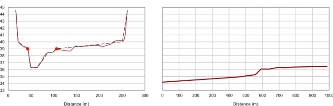
of 1 km and an average slope of 2.3 m km−1. The DEM of the terrain has a mesh size of 1×1 m (Fig. 1).

The bed friction coe_fficient used is the Manning’s n. Three zones are defined with different bed friction values: the main channel,n_ch, the left overbank,n_lob, and the right overbank,nrob(see Fig. 1). Thenvalues over each of the three domains are subjected

15

to uncertainty and therefore are defined as random variables in the model. The vari-ables are assumed to be uncorrelated in this paper, although it is recognized that in fact some correlation may exist between the bed friction values in the defined areas. Nevertheless the methodology exposed in this paper can be applied without di_fficulty to correlated random variables. No spatial variability is considered inside the three

20

defined zones, which corresponds well with the low degree of spatial heterogeneity observed in the reach analyzed.

Di_fferent probability distributions have been used by di_fferent authors to statistically characterise the friction coe_fficient, such as the normal (Cesare, 1991; Mays and Tung, 1992; Horrit, 2006), triangular (Yeh and Tung, 1993), lognormal (USACE, 1986; Liu,

(13)

HESSD

9, 1251–1310, 2012

Title Page

Tables Figures

◭ ◮

Back Close

Full Screen / Esc

Discussion

P

a

per

|

Dis

cussion

P

a

per

|

Discussion

P

a

per

|

Discussio

n

P

a

per

|

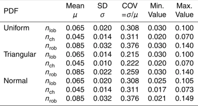
2010) and uniform distributions (Johnson, 1996; Pappenberger et al., 2005). In this pa-per the uniform distribution is selected to examine how point-estimate method pa-performs when distributions have such a high variability. To check the impact of the type of probability distribution of the bed friction on water depth and velocity estimates, also triangular symmetrical and normal distributions have been tested with the 1-D uniform

5

flow model. In the case of the triangular symmetrical distribution the minimum and maximum values are the same as those of the uniform distribution. In the case of the normal distribution a di_fferent truncation has been adopted so the variable is confined exactly between the range [µ_n−2σ_n,µ_n+2σ_n], withµ_nandσ_nthe mean and standard deviation ofn. The probability distributions adopted fornare summarized in Table 1.

10

The study has been undertaken with three di_fferent imposed flows at the upstream end of 200, 300 and 500 m3s−1.

3.2 Numerical flood models

In this section the three hydraulic models used in the study are described.

3.2.1 Uniform flow model

15

The first model used is a uniform flow model that is applied to a simplified geometry (Fig. 2) of the river station RS 768 of the 1-D HEC-RAS model that is described in Sect. 3.2.2. The model assumes an infinite reach length with constant geometry in terms of cross section and slope. The slope of this ideal reach is 2.1 m km−1. This model has been prepared to explore the transfer of variability from bed friction

coef-20

ficient to water depth and velocity functions under ideal conditions, without non-linear perturbations of flow due to changes in geometry. The implicit equation to be solved is the well-known uniform flow formula

Q·S−0.5

=X

i

(14)

HESSD

9, 1251–1310, 2012

Title Page

Tables Figures

◭ ◮

Back Close

Full Screen / Esc

Discussion

P

a

per

|

Dis

cussion

P

a

per

|

Discussion

P

a

per

|

Discussio

n

P

a

per

|

whereQ is the flow (m3s−1), S is the slope of the channel (m m−1),n_i is the random roughness coe_fficient in theith-zone in which the section is divided,A_i is the flow area of thei-zone (m2),Ri is the hydraulic radius (m) of theith-zone andy is the water depth (m). In this case three zones have been defined (i=3): main channel and the left and right overbanks. The simplification of the geometry allows using algebraic expressions

5

forAi(y) andRi(y). The model is implemented in a spreadsheet.

3.2.2 1-D HEC-RAS model

A 1-D HEC-RAS gradually varied flow model of the reach has been prepared. This model is defined by 12 cross sections located along the reach and numbered according to their position in terms of distance in meters to the downstream end (0; 219; 353; 454;

10

558; 591; 640; 694; 737; 768; 773 and 987). Position of the bank stations that define the main channel and the overbanks is consistent with the extent of the zones defined in Fig. 2. At the downstream boundary a normal depth condition is imposed assuming a friction slope of 1.9 m km−1according to the average river slope further downstream. In this model the geometry varies between cross sections. The real cross section at

15

RS 768 compared to the simplified section and the ground profile of the model can be seen in Fig. 2.

3.2.3 2-D Shallow Water Equations model

A 2-D Shallow Water Equations (SWE) flow model has been used to evaluate the system response in terms of water depth and velocities in the domain under analysis.

20

The model solves the well-known 2-D finite volume shallow water equations

∂h ∂t+

∂(hu)

∂x +

∂(hv)

(15)

HESSD

9, 1251–1310, 2012

Title Page

Tables Figures

◭ ◮

Back Close

Full Screen / Esc

Discussion

P

a

per

|

Dis

cussion

P

a

per

|

Discussion

P

a

per

|

Discussio

n

P

a

per

|

∂(hu)

∂t +

∂(hu2)

∂x +

∂(huv)

∂y =−gh

∂(h+z)

∂x +

n2uu2+v20.5

h4/3 +hνT∇

2_u ₍₂₃₎

∂(hv)

∂t +

∂(huv)

∂x +

∂(hv2)

∂y =−gh

∂(h+z)

∂y +

n2vu2+v20.5

h4/3 +hνT∇

2_v ₍₂₄₎

wherehis the flow depth,uandvthe components of the depth averaged flow velocity vector,zthe bed elevation,gthe acceleration due to gravity,nthe Manning’s coe_fficient of roughness and νT the turbulent viscosity. The upstream boundary condition is an

5

imposed inflow and the downstream boundary condition is a stage-discharge relation. This model is implemented in the commercial code GUAD 2D (Inclam and University of Zaragoza, 2008).

The continuous fieldsh,uandv are discretized over a mesh of elements that in this case are squares, but that can have other shapes such as triangles. The governing

10

equations are integrated over each element. The finite volume method combines the main advantages of finite element methods, such as its great geometrical flexibility, with the main advantages of finite di_fference methods, such as its flexibility in the definition of discrete flow variables.

The finite volume method has some disadvantages in the representation of high

15

order derivatives, so they should be used when the viscosity terms can be ignored. The problem is solved over time in GUAD 2D using the Roe approximation based on the local linearization of each Riemann problem between adjacent cells. The time step should be selected small enough to assure stability.

4 Application of the method

20

(16)

HESSD

9, 1251–1310, 2012

Title Page

Tables Figures

◭ ◮

Back Close

Full Screen / Esc

Discussion

P

a

per

|

Dis

cussion

P

a

per

|

Discussion

P

a

per

|

Discussio

n

P

a

per

|

4.1 Uniform flow model – Monte Carlo solutions

The first model used has been the uniform flow model described in previous section. The number of random variables is three which correspond to Manning’s nvalues in main channel and both overbanks. Three flow values are considered, 200, 300 and 500 m3s−1. Three di_fferent probability distributions have been used forn_i according

5

to Table 1, uniform, triangular and normal. The problem has been solved initially with Monte Carlo simulation with 1000 model runs. From these simulations the mean and standard deviation of water depth and velocity at the section have been estimated, and an adaptation of several probability distributions has been attempted, using the statistical tool @RISK (Palisade, 2005).

10

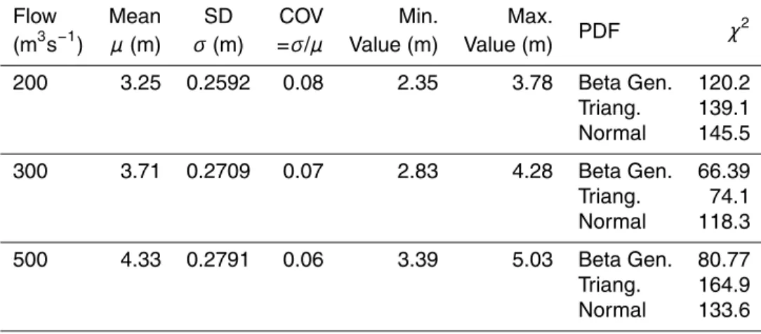
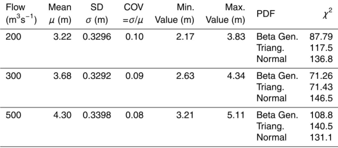
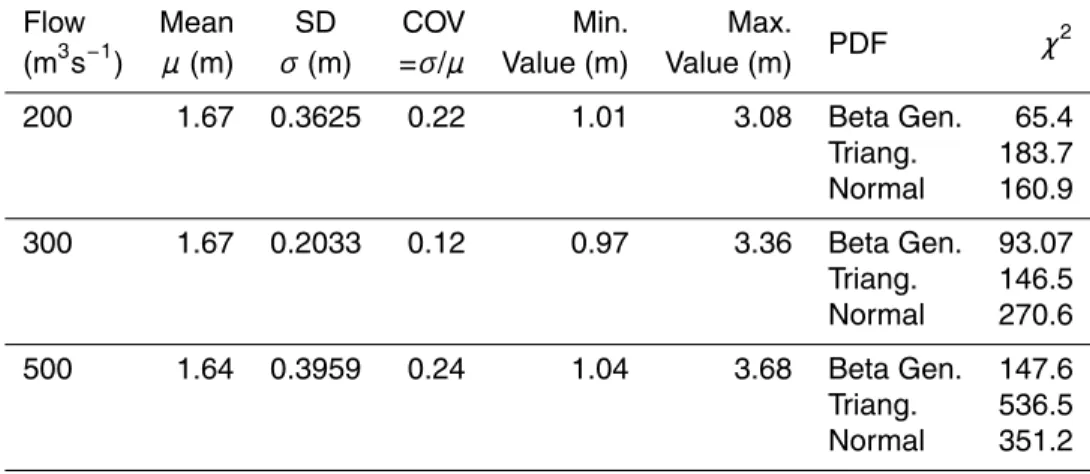
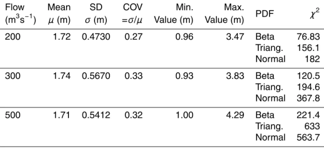
The results for water depth are shown in Tables 2 to 4. In a first step the probability distributions to be fitted have been filtered so only those with lower and upper bounds have been considered, as distributions of ni are bounded as well. The distributions that best fit the data according to the χ2 test are the 4-parameter beta distribution (Beta General) and the 3-parameter triangular distribution. In a second step and for

15

comparison purposes the normal distribution has been selected for fitting. The com-parison of the 4-parameter beta distributions that best fit water depth for case flow 500 m3s−1whenn_i has di_fferent probability distributions is shown in Fig. 3. Graphical comparison of probability density functions suggest that better fitting is obtained when ni are triangular or normal distributed. The best approximation according to χ2 test

20

is obtained whenn_i have triangular distributions. From Fig. 3 it can be seen that the probability distribution of the water depth is not symmetrical, showing some negative skewness. This indicates that symmetrical distributions such as the normal are not a good choice when attempting to describe water depth in a probabilistic way.

A similar analysis has been performed for velocity of flow. The procedure followed

25

(17)

HESSD

9, 1251–1310, 2012

Title Page

Tables Figures

◭ ◮

Back Close

Full Screen / Esc

Discussion

P

a

per

|

Dis

cussion

P

a

per

|

Discussion

P

a

per

|

Discussio

n

P

a

per

|

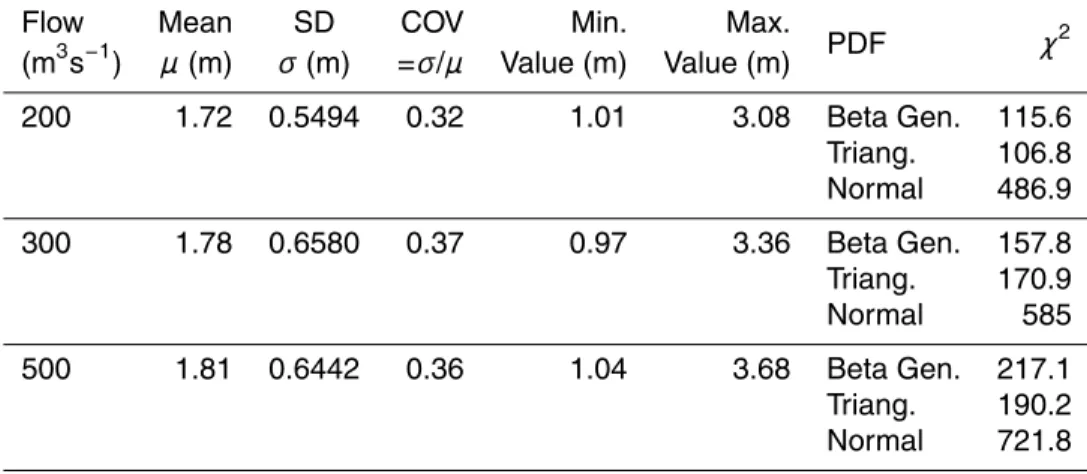
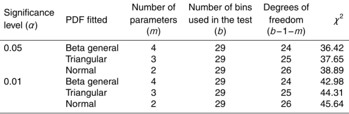
purposes. The results for velocity are shown in Tables 5 to 7. The high values of theχ2 statistic indicates poor fitting in all cases. The comparison of the 4-parameter beta distributions that best fit velocities for flow case 500 m3s−1 whenn_i has di_fferent probability distributions is shown in Fig. 3. The graphic comparison confirms the bad fitting seen in theχ2goodness of fit test. It can be seen that the probability distribution

5

of the velocity is strongly asymmetrical, showing positive skewness. The values of the χ2 statistic for a significance levels of α=0.05 andα=0.01 are shown in Table 8. It can be seen that none of the distributions adapted to water depth and velocity pass the test for a the selected significance levels, thus showing poor fitting, even for this simple hydraulic model.

10

Given that bed friction coe_fficientsni are defined as random variables with bounded distributions, the water depthy derived from the model is another random variable with a bounded distribution, with range [y_MIN,y_MAX]. These limiting values can be calculated straightforwardly from the model. A transformation of the water depth random variable, y, into another random variable,w, is proposed according to

15

w=y_MAX−y (25)

Nowwis a bounded random variable, with positive skewness and confined in the range [0,y_MAX−y_MIN]. The 1000 realisations ofy obtained with Monte Carlo have been trans-formed according to Eq. (25) and new adaptations have been pertrans-formed. Candidate probability distributions have been filtered relaxing the upper bound restriction to let

20

upper unbounded distributions such as the lognormal to be fitted. The results obtained show an improvement in the fitting, particularly when n_i friction values are normally distributed. In Fig. 4 a comparison of lognormal distributions fitted to calculated values is shown. The lognormal distributions fitted do not pass the χ2 goodness of fit test, mainly due to the inaccuracy in the adaptation of the upper tail. This was somehow

25

(18)

HESSD

9, 1251–1310, 2012

Title Page

Tables Figures

◭ ◮

Back Close

Full Screen / Esc

Discussion

P

a

per

|

Dis

cussion

P

a

per

|

Discussion

P

a

per

|

Discussio

n

P

a

per

|

parameters, its mean and standard deviation. The importance of these feature will be addressed later.

The convergence of results of mean and standard deviation values for water depth and velocity obtained with Monte Carlo simulation is shown in Fig. 5 for the case ofn_i uniformly distributed and case flow 500 m3s−1. Similar results have been obtained for

5

the rest of the cases ofni distributions and flow values, so they have not been included here.

4.2 Uniform flow model – point-estimate method approximation

To apply the point-estimate method the first step has been to identify the 2m points where the performance function has to be evaluated, beingmthe number of random

10

variables, which is three in this case. The di_fferent probability distributions of the bed friction coe_fficient considered are symmetrical and roughness values in the three zones defined are assumed to be uncorrelated, although correlation can be easily included as shown in Sect. 2. Applying Eqs. (9) to (12) it can be seen that the two points per variable are located one standard deviation above or below the mean. In this casem=3 and we

15

had 23₌8 points where the performance function had to be evaluated (n₁₊,n₂₊,n₃₊), (n1+,n2+,n3−), (n1+,n2−,n3+), (n1+,n2−,n3−), (n1−,n2+,n3+), (n1−,n2+,n3−), (n1−,

n₂−,n3+), (n1−,n2−,n3−). According to Eqs. (13) and (14) the probability or weight of

each point isP_i=0.125. In Table 9 the corresponding values ofn_i₊ and n_i− for each

zone and distribution are summarized. The mean and variance of the water depth y

20

and velocityv have been calculated with Eqs. (17) to (20), solving the model at the 8 points defined.

The comparison of the results obtained with the three probability distributions of the bed friction coe_fficient considered is shown in Fig. 6. Each dot on the chart corre-spond to a di_fferent flow case. It can be observed that point-estimate gives almost

25

(19)

HESSD

9, 1251–1310, 2012

Title Page

Tables Figures

◭ ◮

Back Close

Full Screen / Esc

Discussion

P

a

per

|

Dis

cussion

P

a

per

|

Discussion

P

a

per

|

Discussio

n

P

a

per

|

estimation is obtained. In summary, point-estimate provides a good approach for mean and standard deviation values of water depth and velocity with a very limited calculation e_ffort.

4.3 1-D HEC-RAS model

A similar procedure has been followed using the 1-D HEC RAS model of the river

5

reach. A di_fference from the previous case is that in this case only uniform probability distributions for bed friction coe_fficients have been considered. The hydraulic model comprises the whole river reach, allowing for changes in section and slope, and so adding non linear e_ffects to the problem with respect to the uniform flow model. Values of water depth and velocity are obtained at the 12 river stations defined in the model.

10

The Monte Carlo analysis has been limited to 100 simulations, which are su_fficient to get a good estimation of the mean and standard deviation values of water depth and velocity, as can be seen by the convergence curves shown in Fig. 7 for cross section at river station RS 768 and flow case 500 m3s−1. In this case the estimated mean water depth isy=4.37 m, and the 95 % confidence interval that corresponds to 100

15

simulations is [4.33; 4.41]. The length of the interval is 0.08 m, which is considered enough accuracy for the purpose of this paper. As a reference, interval lengths of 0.20 and 0.02 m would be expected for 10 and 1000 simulations, respectively. Similar results have been obtained for the other cross sections and flow cases so they are not shown here.

20

The point-estimate method needed only 8 calculations of the hydraulic model for each flow case. The comparison of results obtained with Monte Carlo and point-estimate method is shown in Figs. 8 to 10 for the three flow cases considered. Each dot on the chart corresponds to a different river cross section. It can be seen that the mean depth is well approximated by point-estimate for almost all cross sections.

25

(20)

HESSD

9, 1251–1310, 2012

Title Page

Tables Figures

◭ ◮

Back Close

Full Screen / Esc

Discussion

P

a

per

|

Dis

cussion

P

a

per

|

Discussion

P

a

per

|

Discussio

n

P

a

per

|

and the influence of the whole reach in the flow characteristics of di_fferent sections of the model. The standard deviation of the water depth is reasonably well estimated, showing some scatter for di_fferent flow rates and di_fferent cross sections. For example, at RS 768 the standard deviation of water depth estimated with Monte Carlo has a value of 0.1954 m while point-estimate gives a value of 0.1986 m. The mean velocity is

5

slightly overestimated by point-estimate method though values fit reasonably well with those obtained with Monte Carlo. The standard deviation for velocity shows good per-formance. A comparison of mean and standard deviation of flow profiles for flow case 500 m3s−1is shown in Fig. 11.

Flood uncertainty can be depicted by raster maps of mean and standard deviation

10

of water level values. In Fig. 12 flood inundation maps of the analysed river reach with mean water depths for the three flow cases are shown. In Fig. 13 the raster map of standard deviation of water levels is shown, where the 1-D mathematical structure of the model is highlighted by the alignment of the standard deviation bands parallel to the cross section definition in HEC-RAS model. The pattern reproduced is that of Fig. 11.

15

5 Application to 2-D model

In this section the application of the point-estimate method in combination with a 2-D shallow water equations model is presented. Only uniform probability distributions have been considered for the roughness values of channel and overbanks, in a similar fashion as with 1-D HEC-RAS model.

20

The 2-D hydraulic model had to been run 8 times, according to the 8 combinations of the three random variables point values adopted, for each of the 3 flow cases, so ini-tially 24 runs were needed. To optimize the process a hydrograph with three steps with constant flow rates of 200, 300 and 500 m3s−1has been prepared, reducing the num-ber of model runs from 24 to 8. The duration of each constant flow step has been set

25

(21)

HESSD

9, 1251–1310, 2012

Title Page

Tables Figures

◭ ◮

Back Close

Full Screen / Esc

Discussion

P

a

per

|

Dis

cussion

P

a

per

|

Discussion

P

a

per

|

Discussio

n

P

a

per

|

with the 2-D model implemented in the commercial code GUAD-2D is considerably longer that with 1-D models. Each run of the HEC-RAS model takes less than 1 s while each run of the GUAD-2D model has had an average time duration of 5 h, which makes flood uncertainty analysis with Monte Carlo unfeasible from a practical point of view in engineering. Still, an approximate uncertainty analysis can be performed with the help

5

of the point-estimate method.

The first step has been to perform the calculations with the 2-D hydraulic model at the 8 points where the performance functions have to be evaluated. In this case the performance functions are the water depth and the total velocity at every 1×1 m cell of the model. In this case the total velocity value has been selected though the analysis

10

can be done separately for its components (vX, vY). Series of raster maps with the results of water depths and velocities evaluated for the 8 combinations of roughness coe_fficients are stored in a GIS framework. The mathematical operations defined in Eqs. (18) to (20) have been performed within the GIS using the generated layers with GUAD 2D. The first two moments about the origin of the performance functions are

cal-15

culated at every point of the grid, and from those the expected value and the standard deviation are derived. The flood map with expected values of water depth for the three flow cases is shown in Fig. 14. The standard deviations of water depth can be seen in Fig. 15, where the 2-D mathematical structure of the model becomes clear when compared with equivalent map obtained with HEC-RAS model. The map of mean and

20

standard deviation of velocities of flow is shown in Figs. 16 and 17, respectively. Results from 2-D models can be used to assess the extension of flooded areas with di_fferent severity levels. The flood severity levels are defined in terms of flood depth, velocity and dragging coe_fficient, which is defined as the product of the water depth times the velocity. An example of a chart for flood severity levels is shown in Fig. 18

25

(22)

HESSD

9, 1251–1310, 2012

Title Page

Tables Figures

◭ ◮

Back Close

Full Screen / Esc

Discussion

P

a

per

|

Dis

cussion

P

a

per

|

Discussion

P

a

per

|

Discussio

n

P

a

per

|

For each flow case, every point of the flooded area has been evaluated in terms of water depth, velocity and dragging coe_fficient for the 8 runs of the 2-D model. With the help of GIS tools, the corresponding severity level has been derived for each 1 m2cell using the criteria defined in Fig. 18. The total area for every flood severity level was computed, obtaining 8 di_fferent values for each level. Following the procedure of the

5

point-estimate method the mean and standard deviation of the extension of the flooded area for each severity level has been calculated.

The estimated mean values for each severity level and for the three flow cases are shown in Fig. 19. It can be seen that as flow rate increases the extension of flooded areas with higher severity levels is incremented. The estimated mean values and

stan-10

dard deviations of the extension of the flooded areas for each severity level is shown in Fig. 20 (flow case 200 m3s−1), Fig. 21 (flow case 300 m3s−1) and Fig. 22 (flow case 500 m3s−1). It is interesting to see how the range of variation of extension of flooded areas varies for each severity level, bringing a measure of the uncertainty that can be easily transferred to consequence estimation in a risk analysis context. In the case

15

flow 200 m3s−1 it can be seen that higher uncertainty derived from roughness coe_ffi -cient is present for severity levels low (1) and high (3). For flow case 300 m3s−1low, uniform uncertainty is spread over all severity levels. On the other hand, for flow case 500 m3s−1 a wider band of uncertainty is linked to severity levels high (3) and very high (4).

20

A normalized measure of the amount of uncertainty of a random parameter is the coe_fficient of variation, COV, which is defined as the ratio between the standard devia-tion,σ, and the mean,µ. Values of COV for each severity level for the three flow cases analyzed are depicted in Fig. 23. In engineering practice a small uncertainty would be represented by a COV₌0.05 while considerable uncertainty would be indicated by

25

(23)

HESSD

9, 1251–1310, 2012

Title Page

Tables Figures

◭ ◮

Back Close

Full Screen / Esc

Discussion

P

a

per

|

Dis

cussion

P

a

per

|

Discussion

P

a

per

|

Discussio

n

P

a

per

|

The results in Figs. 20 to 22 show how the uncertainty in bed friction coe_fficient is transferred to flooded areas with di_fferent severity levels. This information is useful in the risk analysis context as flood damage is measured according to the corresponding areas on each severity level. This means that at least some of the uncertainty from the hydraulic model can be added to the estimates of flood damage in the context of risk

5

analysis.

From the point of view of the engineer that has to build a model, information regarding the location of zones with higher variability can be useful to make decisions, such as where to direct the e_fforts for e_fficient model improvement.

6 Conclusions

10

In the context of assessing the uncertainty in flood modelling in a river reach, the re-sults presented have shown the practical applicability of the point-estimate method to perform uncertainty flood analysis, considering the Manning’snroughness coe_fficient as the main source of uncertainty. Reasonable estimates of mean and standard devi-ation values of flood parameters such as water depth and velocity have been obtained

15

with much less e_ffort than with Monte Carlo method using 1-D HEC RAS and a 2-D SWE model implemented in the commercial code GUAD 2D. It has been shown that with a simple variable transformation the water depth parameter can be roughly ap-proximated by a lognormal distribution. Better fitting is observed in the lower tail of the transformed variable which corresponds to the upper tail of the water depth distribution.

20

As the lognormal distribution is fully defined by its mean and variance, a probabilistic characterization can be achieved using PEM.

Flood maps with expected values of water depth and velocity and their associated standard deviations have been obtained implementing the point-estimate calculations within a GIS framework, and flooded areas with di_fferent associated severity levels

25

(24)

HESSD

9, 1251–1310, 2012

Title Page

Tables Figures

◭ ◮

Back Close

Full Screen / Esc

Discussion

P

a

per

|

Dis

cussion

P

a

per

|

Discussion

P

a

per

|

Discussio

n

P

a

per

|

economic losses is achieved using rates linked to the extension of each severity level, uncertainty in the system response is transferred to the consequence evaluation.

The main limitations of point-estimate method are the loss of accuracy if the perfor-mance function cannot be approximated by third order polynomials and the fast growing of the number of calculations needed if the number of random variablesmincreases,

5

rendering the method impracticable for computing time-demanding problems, such as 2-D models. Application to 2-D models, though in need of more research, is promising according to the results obtained.

Though the method presented has some evident advantages such as its sim-plicity and limited e_ffort needed to perform uncertainty analysis of floods with

non-10

probabilistically-oriented 2-D commercial codes, the results obtained should be taken carefully looked at. They should not be deemed as exact values and it should be kept in mind that this method is a practical alternative to more exact methods. It is acknowl-edged that more research is needed in order to set the limits of the applicability of the method and its accuracy in the 2-D models environment, above all when strong

15

non-linearities are present in the model.

The method presented is not always the best choice, but it may be considered by engineers as a useful tool for screening analysis before restoring to more powerful but more costly methods in terms of time and money in the risk analysis context. It is recognized, though, that whenever Monte Carlo application is practically feasible, it is

20

(25)

HESSD

9, 1251–1310, 2012

Title Page

Tables Figures

◭ ◮

Back Close

Full Screen / Esc

Discussion

P

a

per

|

Dis

cussion

P

a

per

|

Discussion

P

a

per

|

Discussio

n

P

a

per

|

References

Aronica, G., Hankin, B., and Beven, K. J.: Uncertainty and equifinality in calibrating distributed roughness coefficients in a flood propagation model with limited data, Adv. Water Resour., 22, 349–365, 1998.

Beven, K. J. and Binley, A.: The future of distributed models: model calibration and uncertainty

5

prediction, Hydrol. Process., 6, 279–298, 1992.

Blad ´e, E., G ´omez, M., and Dolz, J.: Quasi-two dimensional modelling of flood routing in rivers and flood plains by means of storage cells, in: Modelling of Flood Propagation Over Initially Dry Areas edited by: Molinaro, P. and Natal, L., American Society of Engineers, Milan, 1994. Box, G. E. P. and Draper, N. R.: Empirical model building and response surfaces, Wiley, 1987.

10

Cesare, M. A.: First order analysis of open-channel flow, J. Hydraul. Eng.-ASCE, 117, 242–247, 1991.

Christian, J. T. and Baecher, G. B.: Point-estimate method as numerical quadrature, J. Geotech. Geoenviron., 125, 779–786, 1999.

Cobby, D. M., Mason, D. C., and Davenport, I. J.: Image processing of airborne scanning

15

laser altimetry data for improved river flood modelling, ISPRS J. Photogramm., 56, 121–138, 2001.

DEFRA Department for Environment, Food and Rural Affairs: Draft Flood and Water Manage-ment Bill, Welsh Assembly GovernManage-ment, 2009.

Der Kiureghian, A. and Ditlevsen, O.: Aleatory or epistemic? Does it matter?, Special workshop

20

on risk acceptance and risk communication, 26–27, Stanford University, 2007.

Escuder-Bueno, I., Castillo-Rodr´ıguez, J. T., Perales-Momparler, S., and Morales-Torres, A.: SUFRI Methodology for flood risk evaluation in urban areas, Decision guidance for decision maker, Report SUFRI project, WP3, 2011.

European Parliament: Directive 2007/60/EC on the assessment and management of flood

25

risks, Official Journal of the European Union, October 2009.

Gracia, A., God é, L., Crego, E., Arrabal, M. A., Guirado, V., Garc´ıa, G., Lobera, C., Gonz ález, S., and Mart´ınez, E.: Riesgos y cuantificaci ón de da ños por inundaci ón, 5o Congreso In-ternacional de Ordenaci ón del Territorio sobre Gesti ón Compartida de Recursos H´ıdricos Internacionales, Lisboa, 2010 (in Spanish).

30

(26)

HESSD

9, 1251–1310, 2012

Title Page

Tables Figures

◭ ◮

Back Close

Full Screen / Esc

Discussion

P

a

per

|

Dis

cussion

P

a

per

|

Discussion

P

a

per

|

Discussio

n

P

a

per

|

Hoek, E.: Practical Rock Engineering, online course, available at: http://www.rocscience.com/ education/hoeks corner, 2007.

Horrit, M. S.: A linearized approach to flow resistance uncertainty in a 2-D finite volume model of flood flow, J. Hydrol., 316, 13–27, 2006.

Inclam-University of Zaragoza, Departamento de mec ´anica de fluidos, Guad 2D Flow Software,

5

Manual de Usuario, V1.1, 2011.

Johnson, P. A.: Uncertainty of Hydraulic Parameters, J. Hydraul. Eng.-ASCE, 122, 112–114, 1996.

Kelly, K. S. and Krzysztofowicz, R.: A bivariate meta-Gaussian density for use in hydrology, Stoch. Hydrol. Hydraul., 11, 17–31, 1997.

10

Liu, D. S. and Matthies, H. G.: Uncertainty quantification with spectral approximations of a flood model, IOP Conf. Ser.: Mater. Sci. Eng., 10, 012208, doi:10.1088/1757-899X/10/1/012208, 2010.

Mason, D. C., Cobby, D. M., Horrit, M. S., and Bates, P. D.: Flood plain friction parameteri-sation in two-dimensional river flood models using vegetation heights derived from airborne

15

scanning laser altimetry, Hydrol. Process., 17, 1711–1732, 2003.

Mays, L. W. and Tung, Y. K.: Hydrosystems engineering and management, McGraw-Hill, New York, 1992.

Palisade Corporation: @RISK software, User’s Manual, available at: http://www.palisade.com/ support/manuals.asp, 2005.

20

Pappenberger, F., Beven, K., Horrit, M., and Blazkova, S.: Uncertainty in the calibration of effective roughness parameters in HEC-RAS using inundation and downstream level obser-vations, J. Hydrol., 302, 46–49, 2005.

Pappenberger, F., Frodsham, K., Beven, K., Romanowicz, R., and Matgen, P.: Fuzzy set ap-proach to calibrating distributed flood inundation models using remote sensing observations,

25

Hydrol. Earth Syst. Sci., 11, 739–752, doi:10.5194/hess-11-739-2007, 2007.

Romanowicz, R. and Beven, K.: Dynamic real-time prediction of flood inundation probabilities, Hydrolog. Sci. J., 43, 181–196, 1998.

Rosenblueth, E.: Two-point estimates in probabilities, Appl. Math. Model., 5, 329–335, 1981. Rubinstein, R. Y.: Simulation and the Monte Carlo Method, John Wiley & Sons, 1981.

30

Sarino and Serrano, S. E.: Development of the instantaneous unit hydrograph using stochastic differential equations, Stoch. Hydrol. Hydraul., 4, 151–160, 1990.

(27)

HESSD

9, 1251–1310, 2012

Title Page

Tables Figures

◭ ◮

Back Close

Full Screen / Esc

Discussion

P

a

per

|

Dis

cussion

P

a

per

|

Discussion

P

a

per

|

Discussio

n

P

a

per

|

rainfall runoffmodelling, Int. J. River Basin Manage., 6, 109–122, 2008.

UNWWAP United Nations World Water Assessment Programme: Global trends in water-related disasters, an insight for policymakers, United Nations, 2009.

US Army Corps of Engineers: Hydraulic Engineering Center, Accuracy of computed water surface profiles, Technical report, Hydraulic Engineering Center, Davis, Calif, 1986.

5

US Army Corps of Engineers: HEC-RAS River Analysis System User’s Manual, available at: http://www.hec.usace.army.mil, 2002.

US Army Corps of Engineers: HEC-FDA Flood Damage Reduction Analysis User’s Manual, available at: http://www.hec.usace.army.mil/software/hec-fda/documentation/CPD-72 V1.2. 4.pdf, 2008.

10

Wohl, E. E.: Uncertainty in flood estimates associated with roughness coefficient, J. Hydraul. Eng.-ASCE, 124, 219–223, 1998.

Yeh, K. C. and Tung, Y. K.: Uncertainty and sensitivity analysis of pit-migration model, J. Hy-draul. Eng.-ASCE, 119, 262–283, 1993.

Yue, S., Taha, B. M., Ouarda, J., Bobe ´e, B., Legendre, P., and Bruneau, P.: Approach for

15

(28)