www.hydrol-earth-syst-sci.net/19/913/2015/ doi:10.5194/hess-19-913-2015
© Author(s) 2015. CC Attribution 3.0 License.
Climate change impacts on the seasonality and generation
processes of floods – projections and uncertainties for
catchments with mixed snowmelt/rainfall regimes
K. Vormoor1, D. Lawrence2, M. Heistermann1, and A. Bronstert1
1Institute of Earth and Environmental Science, University of Potsdam, Postdam, Germany 2Norwegian Water Resources and Energy Directorate (NVE), Oslo, Norway
Correspondence to:K. Vormoor ([email protected])
Received: 22 May 2014 – Published in Hydrol. Earth Syst. Sci. Discuss.: 13 June 2014 Revised: 14 January 2015 – Accepted: 22 January 2015 – Published: 12 February 2015
Abstract.Climate change is likely to impact the seasonality and generation processes of floods in the Nordic countries, which has direct implications for flood risk assessment, de-sign flood estimation, and hydropower production manage-ment. Using a multi-model/multi-parameter approach to sim-ulate daily discharge for a reference (1961–1990) and a fu-ture (2071–2099) period, we analysed the projected changes in flood seasonality and generation processes in six catch-ments with mixed snowmelt/rainfall regimes under the cur-rent climate in Norway. The multi-model/multi-parameter ensemble consists of (i) eight combinations of global and regional climate models, (ii) two methods for adjusting the climate model output to the catchment scale, and (iii) one conceptual hydrological model with 25 calibrated parame-ter sets. Results indicate that autumn/winparame-ter events become more frequent in all catchments considered, which leads to an intensification of the current autumn/winter flood regime for the coastal catchments, a reduction of the dominance of spring/summer flood regimes in a high-mountain catchment, and a possible systematic shift in the current flood regimes from spring/summer to autumn/winter in the two catchments located in northern and south-eastern Norway. The changes in flood regimes result from increasing event magnitudes or frequencies, or a combination of both during autumn and winter. Changes towards more dominant autumn/winter events correspond to an increasing relevance of rainfall as a flood generating process (FGP) which is most pronounced in those catchments with the largest shifts in flood season-ality. Here, rainfall replaces snowmelt as the dominant FGP primarily due to increasing temperature. We further analysed
the ensemble components in contributing to overall uncer-tainty in the projected changes and found that the climate projections and the methods for downscaling or bias correc-tion tend to be the largest contributors. The relative role of hydrological parameter uncertainty, however, is highest for those catchments showing the largest changes in flood sea-sonality, which confirms the lack of robustness in hydrolog-ical model parameterization for simulations under transient hydrometeorological conditions.
1 Introduction
The hydrological cycle is likely to intensify due to climate change (IPCC, 2007; Seneviratne et al., 2012), and a recent study indicates that global warming has caused more intense precipitation over the last century on the global scale (Ben-estad, 2013). These changes will, in turn, have direct impli-cations for flood risk. For mountainous and Nordic regions, changes in the ratio of rainfall and snowfall due to tempera-ture rise are of special interest since they have direct impli-cations for flood seasonality and for the dominant processes generating flood discharge.
system-atic trends in spring flood magnitudes are yet detected (Wil-son et al., 2010). The same study found, however, a strong trend towards earlier spring floods at many stations. This is likely due to the observed increase in mean annual temper-ature during the last century, which has been reported to be 0.8◦C, with the strongest decadal temperature rise during the
spring season (Hanssen-Bauer et al., 2009).
Climate projections for Norway for the end of the 21st cen-tury indicate increasing temperatures (2.3–4.6◦C) and
pre-cipitation (5–30 %) with the largest temperature increase dur-ing winter in northern Norway, and the largest precipita-tion increase during autumn and winter on the west coast (Hanssen-Bauer et al., 2009). Extreme precipitation is also likely to increase for all seasons across the whole of Norway (Beniston et al., 2007; Hanssen-Bauer et al., 2009; Senevi-ratne et al., 2012), although such projections are highly un-certain (Fowler and Ekström, 2009). Changes in temperature and precipitation regimes will have direct implications for the snow regime in Norway. For mountainous areas and in northern Norway where mean winter temperature is a few degrees below 0, snow depth is observed to have increased in recent decades (Dyrrdal et al., 2013) and climate projections suggest further increases until 2050 (Hanssen-Bauer et al., 2009). In other parts of Norway snow depths are projected to decrease. Towards the end of the 21st century, a decrease in snow depths and a shorter snow season are projected for the whole of the country due to temperature rise.
For the Nordic countries, several previous studies have investigated the hydrological impacts of climate change (e.g. Andréasson and Bergström, 2004; Roald, 2006; Beldring et al., 2008; Veijalainen et al., 2010; Lawrence and Hisdal, 2011; Lawrence and Haddeland, 2011). For Norway, Lawrence and Hisdal (2011) studied the changes in flood fquency in 115 Norwegian catchments and found coherent re-gional patterns of directional change in flood magnitudes un-der a future climate: the magnitudes of the 200-year flood, for example, is likely to increase in catchments in western and much of coastal Norway where flood generation is dominated by autumn/winter rainfall, while magnitudes are expected to decrease in the snowmelt-dominated catchments in inland ar-eas and parts of northern Norway. This regional pattern re-flects systematic changes in climate forcing, which lead to changes in hydrological flooding in terms of both seasonal prevalence and generation process (rainfall vs. snowmelt). There are, however, many catchments which are transitional between rainfall-dominated vs. snowmelt-dominated flood regimes, and interpretation of the likely direction of change in the magnitude of future floods is more difficult. In addi-tion, such catchments may be subject to a shift in the flood season under a future climate. Considering the uncertainty in the projections for future (extreme) precipitation and sub-sequent flooding conditions (Bronstert et al., 2007), Blöschl et al. (2011) argue that seasonal change in the distribution of floods is the key to understanding climate change impacts on flooding rather than changes in flood magnitudes and
fre-quencies. Changes in the underlying flood generating pro-cesses (FGPs) are correspondingly important for interpreting the direction (i.e. increase vs. decrease) of climate change impacts on future floods. Therefore, we aim to study in detail the changing role of rainfall and snowmelt under future cli-mate scenarios to aid in understanding flood regime changes in catchments which already show mixed snowmelt/rainfall flood regimes in today’s climate.
For practical purposes, changes in flood seasonality have implications for future flood risk assessments, design flood estimations, and hydropower production management. In Norway, where hydropower represents about 96 % of the to-tal electricity production, flood seasonality impacts reservoir management and accordingly hydropower production. In ad-dition, design flood estimates for dam safety require that the season for the highest flood risk is assessed (e.g. Midttømme et al., 2011) and changes in the dominant flood season under a future climate have significant implications for these as-sessments. Despite the relevance of this issue, there has not yet been a detailed investigation of climate change impacts on future flood seasonality and the process-related factors contributing to those changes in Norway.
In this study, we investigate the impact of climate change on flood seasonality and the related FGPs in six Norwe-gian catchments representing different geographical and cli-matological conditions. The catchments were selected such that both rainfall and snowmelt sometimes play a role in the generation of high-flow events under the current climate; we investigate how the balance between these two flood generating factors changes. We apply a multi-model/multi-parameter ensemble to develop a range of hydrological pro-jections which allows us to consider some of the uncertainties associated with such an analysis (e.g. Hall et al., 2014). The multi-model/multi-parameter ensemble used here consists of eight combinations of global and regional climate models (GCM/RCM combinations), two methods for locally adjust-ing the climate model output data to the catchment scale, and hydrological modelling implemented with the HBV model based on 25 calibrated parameter sets. Our particular re-search questions are (1) how might the existing patterns of flood seasonality change under a future climate? (2) How are shifts in seasonality related to changes in the magnitude vs. changes in the frequency of events? (3) Are changes in flood seasonality associated with changes in the dominant FGPs? (4) What is the relative importance of the different ensemble components in contributing to the overall variance as a measure of the uncertainty in the projected changes?
2 Study area
2.1 Climate and runoff regimes in Norway
pat-tern of temperature and precipitation regimes in Norway. The mean annual temperature varies from 7.7◦C at the
south-western coast to about −3◦C in the inland areas of
northern Norway and the high-altitude areas in central Nor-way (Hanssen-Bauer et al., 2009). Mean annual precipitation varies from about 300 mm in north-eastern and central Nor-way to more than 3500 mm in western NorNor-way (Hanssen-Bauer et al., 2009). Seasonally, western Norway receives the largest precipitation volumes during the autumn and winter months, while the more inland region in the east receives these during the summer.
Mean annual runoff generally reflects the pattern of mean annual precipitation, and runoff coefficients tend to be high due to low evapotranspiration. However, due to differences in the temperature regime, snowpack volumes and the snow season vary considerably across the country, which leads to differences in the regional importance of snowmelt as a runoff generation process. Hence, two basic patterns in runoff regimes can be distinguished in Norway: (i) regions in inland and northernmost Norway with prominent high flows during spring and summer predominantly due to snowmelt, and (ii) regions in western Norway and in coastal regions with prominent high flows during autumn and winter pre-dominantly due to rainfall. There are, though, numerous vari-ations reflecting local climate as well as transitional, mixed, regimes. In addition, catchments with sources in high moun-tain areas can experience peak flows in late summer, due to glacier melt. A comprehensive classification of runoff regimes based on the seasonal occurrence of monthly high and low flows is given by Tollan (1975) and reviewed in Gottschalk et al. (1979). This classification defines five types of flood regimes for the Nordic countries and give detailed distinctions between possible combinations of high-flow and low-flow periods. However, in order to develop a broad pic-ture of flood seasonality, it is most useful to apply the simple distinction between two high-flow seasons (spring/summer vs. autumn/winter) and to distinguish rainfall vs. snowmelt as the most fundamental flood generation processes.
2.2 Study catchments
Changes in flood seasonality and the FGPs were investi-gated in six catchments distributed across Norway: Krins-vatn, FustKrins-vatn, ØvreKrins-vatn, Junkerdalselv, Atnasjø, and Kråk-foss (Fig. 1). These catchments represent some of the vari-ability in climate conditions across the country. The focus in this work, however, is on catchments which already exhibit some tendency for both snowmelt- and rainfall-dominated flood regimes. Therefore, a full range of climatic conditions is not represented nor are some regions (e.g. western and southern coastal Norway) included in this analysis. In ad-dition, the sample includes only catchments of moderate size which are suitable for hydrological modelling with a daily time step.
The catchments considered are largely unaffected by damming or regulation (Petterson, 2004), and anthropogenic land use (changes) can be neglected since land use consti-tutes only between 0 and 1 % of land cover in all catch-ments except Kråkfoss (11 %). The catchcatch-ments are included in the benchmark data set for climate change studies for Norway and are classified as suitable for daily analyses of flood discharge (Fleig et al., 2013). The six catchments are mesoscale catchments and vary in size from 207 km2 (Krins-vatn) to 526 km2 (Fustvatn). Further catchment characteris-tics including elevation, land cover, as well as mean annual precipitation and runoff are given in Table 1. Figure 1 dis-plays flood roses to illustrate the magnitudes of the annual maximum floods (AMFs) from observed daily series by their Julian date of occurrence. These plots indicate the flood sea-sonality for the six catchments for the period 1961–1990 (ex-cept for Kråkfoss where the observed time series begins in 1966).
Although Krinsvatn and Fustvatn have the lowest ele-vations amongst the catchments, they receive a consider-ably higher annual precipitation (2291 and 3788 mm, re-spectively) due to their coastal locations. Correspondingly, the catchments have large average annual runoff values, and both the majority of and the largest AMFs occur during late autumn and winter, representing rainfall-dominated flood generation. However, both catchments are also subject to snowmelt floods, as indicated by the comparatively smaller events occurring during spring.
Øvrevatn, Junkerdalselv and Atnasjø show the highest median elevation and elevation ranges, but differ consider-ably with respect to annual precipitation and runoff volumes. Øvrevatn and Atnasjø, though being the highest catchments within this comparison, receive considerably less precipita-tion (832 and 840 mm, respectively) due to their rain shadow locations. Junkerdalselv, being located further inland near the Swedish border, is not directly influenced by rain shadow ef-fects and has annual precipitation and runoff volumes that are about 3 times larger than at Øvrevatn and Atnasjø. Be-cause of the temperature regime, all three catchments receive a large portion of the annual precipitation as snow so that the majority of and the largest AMFs occur during spring and summer (May–July, Fig. 1), with snowmelt as the dominant FGP.
Annual Maximum8Floods
20 60 100
Jan
Feb
Mar
Apr
May
Jun Jul Aug Sep Oct
Nov Dec
Krinsvatn81961−2008
20 40
Jan
Feb
Mar
Apr
May
Jun Jul Aug Sep Oct
Nov Dec
Fustvatn81961−2008
20 40
Jan
Feb
Mar
Apr
May
Jun Jul Aug Sep Oct
Nov Dec
Øvrevatn81961−2008
10 20 30
Jan
Feb
Mar
Apr
May
Jun Jul Aug Sep Oct
Nov Dec
Junkerdalselv81961−2008
5 15 25
Jan
Feb
Mar
Apr
May
Jun Jul Aug Sep Oct
Nov Dec
Kråkfoss81966−2008
5 15 25
Jan
Feb
Mar
Apr
May
Jun Jul Aug Sep Oct
Nov Dec
Atnasjø81961−2008
Figure 1.The location of the six study catchments and their current flood regime demonstrated by flood roses indicating the magnitude and
timing of observed annual maximum floods. Values are given as specific discharge (mm day−1). Note that secondary annual flood peaks can
occur during contrasting seasons.
Table 1.Characteristics of the six study catchments.
Catchment Krinsvatn Fustvatn Øvrevatn Junkerdalselv Atnasjø Kråkfoss property
Area (km2) 207 526 525 420 463 433
Median elevation 349 436 841 835 1205 445
(m a.s.l.)
Elevation range 87–629 39–812 145–1636 117–1703 701–2169 105–803 (m a.s.l.)
Average annualP 2291 3788 832 3031 840 2092
(mm)
Average annualQ 1992 3017 564 2722 672 1798
(mm)
Land cover, % 8 6 10 0 2 4
lake
Land cover, %
0 <1 4 1 <1 0
glacier
Land cover, % 20 38 23 25 20 76
forest
Land cover, % 9 5 1 1 2 5
marsh and bog Land cover, %
57 37 57 63 69 0
sparse vegetation above treeline Anthropogenic
0.4 0.0 0.7 0.5 0.4 11.2
most of the catchments dominated by rainfall-induced flood-ing have periods in which a transient snow cover also may contribute to runoff during rainfall. Therefore, for this study it is useful to define a third FGP (“rainfall+snowmelt”),
which occurs to varying degrees in all six catchments con-sidered.
The dominant land cover types in the six catchments are either exposed (crystalline) bedrock with sparse vegetation above tree line (Atnasjø, 69 %; Junkerdalselv, 63 %; Krins-vatn, 57 %; ØvreKrins-vatn, 57 %) or boreal forest (Kråkfoss, 76 %; Fustvatn, 38 %). Soils in all catchments are rather thin and poorly developed, and large, regional groundwater storage in aquifers is virtually non-existent due to the crystalline bedrock. However, in most catchments, surface water in the form of lakes, marshes and bogs can lead to water retention and, in some cases, significant attenuation of flood peaks.
3 Data and methods 3.1 Modelling strategy
The analyses of changes in flood seasonality and their as-sociated FGPs are based on a multi-model/multi-parameter ensemble approach consisting of (i) eight GCM/RCM com-binations, (ii) two methods for adjusting the temperature and precipitation outputs of the climate models at the catchment scale, and (iii) the HBV hydrological model with 25 different parameter sets for considering hydrological parameter uncer-tainty. It has become good practice to include more than one model for each member within the model chain to derive a range of possible projections and to allow drawing conclu-sions about the uncertainty that is associated by such ap-proaches. We have only used one hydrological model in our ensemble setup; this is supported by Velázquez et al. (2013), who conclude that the use of multiple hydrological models in climate impact studies is important for the study of low flows and means, but not for high flows, as various lumped and distributed models lead to very similar results. Moreover, the HBV model has been widely applied in the Nordic coun-tries since it represents a suitable conceptual representation of the dominant runoff generating processes and does not im-pose excessive data requirements. The following subsections describe the individual components of the ensemble in more detail.
3.2 Climate projections
The climate projections for precipitation and temperature chosen for the hydrological simulations are based on eight GCM/RCM combinations (Table 2) from the EU FP6 EN-SEMBLES project (van der Linden and Mitchell, 2009). The spatial resolution of all RCMs considered is 0.22◦
(approxi-mately 25 km), and projections of daily values are available for the period 1950–2099. Within this study, two periods are compared: a reference period (1961–1990) for which the
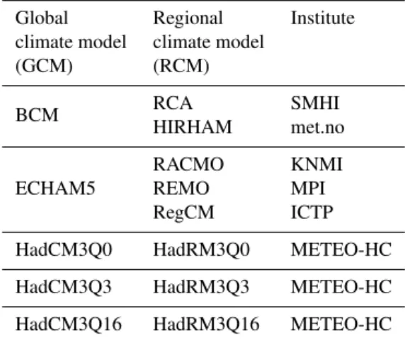
Table 2.The GCM/RCM combinations from ENSEMBLES used
for the hydrological projections. The full names of the institute ab-breviations are SMHI – Swedish Meteorological and Hydrological Institute, met.no – the Norwegian Meteorological Institute, KNMI – The Royal Netherlands Meteorological Institute, MPI – Max Planck Institute for Meteorology (Germany), ICTP – International Cen-tre for Theoretical Physics (Italy), METEO-HC – The Met Office Hadley Centre (UK).
Global Regional Institute climate model climate model
(GCM) (RCM)
BCM RCAHIRHAM SMHImet.no
ECHAM5
RACMO KNMI
REMO MPI
RegCM ICTP
HadCM3Q0 HadRM3Q0 METEO-HC
HadCM3Q3 HadRM3Q3 METEO-HC
HadCM3Q16 HadRM3Q16 METEO-HC
GCM/RCM combinations are driven by the IPCC-AR4 sce-nario C20, and a future period (2071–2099) for which the cli-mate model combinations are driven by the SRES A1B sce-nario, which represents intermediate greenhouse gas emis-sions until the end of the 21st century (IPCC, 2000, 2007). We only focus on the far future period since the change sig-nals are more pronounced by this time. We selected the eight RCMs from ENSEMBLES that are nested within as many different GCMs as possible to minimize the interdependency between the climate model outputs used (Sunyer et al., 2013). 3.3 Local adjustment methods (LAMs)
It is widely acknowledged that the RCM outputs for the vari-ables of interest (in our case precipitation and temperature) are biased due to limited process description, biased fluxes at the RCM margins and insufficient spatial resolution relative to the catchment scale (Engen-Skaugen et al., 2007). There-fore, data post-processing is necessary to bridge the gap be-tween the large-scale climate model and the local hydrolog-ical processes (e.g. Maraun et al. 2010; Chen et al., 2011). Considerable progress has been made during recent years re-garding the development and improvement of such methods and Hanssen-Bauer et al. (2005), Fowler et al. (2007), Ma-raun et al. (2010), and Teutschbein and Seibert (2012) give comprehensive reviews on available approaches.
ex-panded downscaling (Bürger, 1996; Bürger et al., 2009) which is a type of statistical downscaling.
3.3.1 Empirical quantile mapping (EQM)
EQM is a bias correction method that seeks a transfer func-tion (h) to adjust RCM data so that it is in better agreement
with observations. By adjusting the quantiles of the biased RCMs (xm) to those of the locally observed data (xo), the bias-corrected distribution of xmshould match the distribu-tion ofxo, such that
xo=h (xm)=Fo−1(Fm(xm)) , (1)
whereFm is the empirical cumulative distribution function (eCDF) of xm, and Fo−1 is the inverse eCDF (the quantile
function) corresponding toxo. Based on the assumption that
the shortcomings of the climate model are the same for the reference and future periods (van Roosmalen et al., 2011) and that the transfer function is stationary in time (Maraun et al., 2010), the function is applied to bias-correct projections from RCMs for both the reference and future periods.
For Norway, Gudmundsson et al. (2012) found that non-parametric transfer methods (as EQM) performed best for the bias correction of precipitation compared to parametric and distribution-derived transformations. For temperature, we found the same ranking though the differences are not as large as for precipitation. Therefore, EQM was consid-ered as a suitable LAM for the correction of daily precipita-tion and temperature values for this study. The method was implemented as an add-on package (qmap; Gudmundsson, 2014) for the statistical programming environment R (R Core Team, 2012). Bias correction was performed on daily values for the full year, without distinguishing seasons, following work of Piani et al. (2009) which illustrated that the cor-rection without seasonal subsampling performs remarkably well.
3.3.2 Expanded downscaling (XDS)
XDS is a statistical downscaling approach and, as such, it maps large-scale atmospheric fields (the predictors – x)
to local data (the predictands – y). XDS has been
ap-plied for various purposes, e.g. for early flood warning (Bürger et al., 2009), downscaling extreme precipitation pro-jections (Dobler et al., 2013), and hydrological impact stud-ies (Dobler et al., 2012a).
At its core, XDS is based on multiple linear regression (MLR) which leads to minimizing the least square errors. The drawback of MLR, however, is that local climate vari-ability will be smoothed significantly, which has strong im-plications for the simulation of extremes. To overcome this limitation, XDS adds an additional condition for retaining local co-variability between the variables:
XDS=argmin
Q ||xQ−y||,subjected toQ
′
x′xQ=y′y, (2)
such that XDS is the solution of the error-minimizing ma-trixQ(xQ−y) which is found amongst those that preserve
the local covariance (Q′
x′xQ=y′y). This approach is
sup-posed to improve the estimation of extreme events, at the cost of a larger mean error as compared to conventional MLR.
For the present study, we used humidity, wind fields, tem-perature, and precipitation characteristics as predictor fields. XDS was calibrated on the RCM atmospheric fields driven by the ECMWF ERA-40 reanalysis (Uppala et al., 2005) for the period 1961–1980, and then applied to downscale the RCM outputs for the reference and future scenarios. 3.4 The HBV model
The analysis of climate change impacts at the catchment scale is based on daily streamflow simulated by the lumped, conceptual HBV model (Bergström, 1976, 1995), forced by the locally adjusted RCM data. In this study we apply the “Nordic” version of the model (Sælthun, 1996), which incor-porates a snow module with 10 equal area height zones, such that snow accumulation and melting has a semi-distributed structure. For each equal area height zone, snow accumula-tion and melting is calculated individually, and the mean is finally used to represent the snow dynamics for each catch-ment. The principal advantage of the HBV model relative to more physically based models are that it only requires pre-cipitation and temperature as climatological input. These are given as catchment mean values for the catchment centroid. Input data for precipitation and temperature are modified for the snow routine by three parameters defining the precipita-tion altitude gradient, and the temperature gradients for dry and wet days, respectively.
The HBV model was calibrated for each catchment using daily-averaged discharge data. Excepting Kråkfoss, where observed data are only available since 1966, the entire ref-erence period (1961–1990) was used for model calibration. The use of such a long calibration period increases the chance that all relevant processes are covered (Merz et al., 2009). The model calibration uses the dynamically dimensioned search (Tolson and Shoemaker, 2007) (DDS) which is a global optimization algorithm for the calibration of multi-parameter models. A modified version of the Nash–Sutcliffe efficiency (NSE) was used as the objective function so as to focus on matching the high-flow events
NSEw=1− n
P
i=1
Qobs(Qsim−Qobs)2
n
P
i=1
Qobs Qsim−Qobs2
, (3)
discharge. A mismatch between high observed and simulated discharges is, therefore, penalized proportionally to the ob-served discharge value.
To account for parameter uncertainty, 25 best-fit parameter sets were identified and included for the hydrological simu-lations. Fifteen free parameters were subjected to the cali-bration by DDS, which was setup to 1200 model calls. The best-performing parameter set was taken directly from the DDS calibration. The remaining 24 parameter sets were iden-tified by a subsequent Monte Carlo simulation with another 1200 model calls using a narrowed range in the parameter values which was defined by the range of parameter values of the 36 (3 %) best parameter sets identified by DDS. In that way, the effects of interdependency between the parameter sets are minimized.
3.5 Change analysis
The extreme events of the daily streamflow simulations were extracted using a peak over threshold (POT) approach, which leads to a more comprehensive selection of events (in terms of timing and flood processes) compared the block maxi-mum method (i.e. AMF) (Lang et al., 1999). The threshold was set to the 98.5 streamflow percentile for both the con-trol and future periods. Independency of events was achieved by enforcing that (i) only one event can occur within twice the normal flood duration (which is catchment specific) and (ii) that only the largest event will be considered if more than one peak is identified within that time period. The normal flood duration has been derived, for each of the six catch-ments considered, by a simple experiment using the HBV model. Each catchment was artificially drained to baseflow conditions before twice the amount of annual rainfall was added to completely saturate the catchment again. Concen-tration and recession time to baseflow were estimated from the resulting hydrographs. The normal flood duration for the catchment was then defined as the sum of the concentration and recession times.
3.5.1 Changes in flood seasonality
Detected POT events were divided into two seasons reflect-ing the basic flood regimes described in Sect. 2.1: (i) the spring/summer period from March to August, which is asso-ciated with snowmelt as an important FGP under the current climate, and (ii) the autumn/winter period from September to February, which is associated with rainfall as the most im-portant FGP. To quantify the seasonality of flood events, we define a seasonality indexSD:
SD=POTSep–Feb
POTall −
POTMar–Aug
POTall , (4)
where the first term describes the ratio between the flood peaks (m3s−1) of the POT events occurring within the period
September–February over all POT events, and the second
term describes the ratio between the POT events occurring within March–August over all POT events. The index ranges from−1 to+1: negative numbers indicate dominant events
during spring/summer while positive numbers indicate domi-nant events during autumn/winter.SDwas estimated for each ensemble member for both the reference and the future peri-ods. The difference inSDbetween the future and the refer-ence periods is an indicator of changes in flood seasonality. In addition, the magnitudes and frequencies of the detected spring/summer and autumn/winter events were analysed for the reference and the future periods. The changes in magni-tudes and relative frequencies of the events within each sea-son aid in explaining changes in flood seasea-sonality.
3.5.2 Changes in FGPs
Each POT event was analysed to determine the dominant contribution to flood discharge. This contribution has been inferred from the runoff components simulated by the HBV model. A simple water balance approach was used to classify the events into floods generated by (i) “rainfall”, (ii) “rain-fall+snowmelt” and (iii) “snowmelt”. The classification is
based on the relative contribution of the volumes of rainfall and snowmelt to the flood event discharge: an event was clas-sified as rainfall if the contribution of rainfall was larger than two-thirds, and classified as snowmelt if rainfall contribution was smaller than one-third. Other events were classified as rainfall+snowmelt. Note that there exist more detailed
ap-proaches for classifying types of flood processes, including the use of various process indicators (e.g. flood timing, storm duration, rainfall depth, snowmelt, catchment states), as sug-gested by Merz and Blöschl (2003). The classification pro-posed here, however, is very easy to apply and fully suitable for our analyses, given the broad distinction between rainfall and snowmelt flood generation that we are using in this work. In addition, the required runoff components can be readily extracted from the output of the HBV model.
Events were identified using a tool implemented in the R add-on package seriesdist (https://bitbucket.org/heisterm/ seriesdist), which enables the detection of both flood peaks and their event-specific flood duration. In order to also ac-count for the antecedent conditions in the catchment, the de-tected flood duration time of the core event was extended by adding the catchment-specific recession time (found in the definition of the normal flood duration) before the onset of the flood. The classification approach was then applied to the extended flood duration time such that all relevant contribu-tions to the peak flow are considered.
Two statistics were applied to identify changes in the FGPs: (1) the ratios of rainfall-, rainfall+snowmelt- and
of the rainfall-, rainfall+snowmelt- and snowmelt-generated
events were calculated for both periods to illustrate changes in the annual distribution and mean timing of the events. The circular mean Julian dates of occurrence for the events with respect to each FGP are converted to mean radians (2)
esti-mated from the Julian date of occurrenceDfor each eventi:
2i =
D2π
365 , (5)
where the Julian dateD=1 is for 1 January andD=365 for
31 December. Thexandy coordinates for the mean date as
an angular value are derived from the sample ofnevents for
each FGP group:
x=1
n
n
X
i=1
cos2i, (6)
y=1
n
n
X
i=1
sin2i, (7)
2=tan−1
y x
. (8)
This approach was introduced by Bayliss and Jones (1993) and Burn (1997), and has been recently applied by Parajka et al. (2010) and Köplin et al. (2014). Note that these authors also estimate the variability of the date of occurrence. In this study, this is illustrated using the circular kernel density func-tions.
3.6 Sources of uncertainty
The range of all ensemble realizations provides a measure of the overall uncertainty represented by the ensemble, given that each projection is assumed to be equally likely. Similar to Déqué et al. (2007, 2011), the mean variance σ2ensemble (as a measure of uncertainty) of the entire ensemble is here defined as the additive mean variances from the ensemble components:
σ2ensemble=σ2GCM/RCM+σ2LAM+σ2HP. (9)
We exemplify the computation of mean variances from the ensemble components for the hydrological model parame-terization (σ2HP): for each combinationi out ofnpossible
combinations of GCM/RCMs and LAMs, we compute the varianceσHP,i subject to 25 parameter sets of the hydrolog-ical model. Then, we compute σ2HP as the mean over all
σHP,i...n.σ2GCM/RCMandσ2LAMare computed accordingly. This approach was used to identify the fractional uncer-tainty emerging from the different sources within the model chain for three variables: (i) the change in the index SD,
(ii) the change in the median magnitude of the POT events, and (iii) the change in the fraction of snowmelt- over rainfall-generated events.
4 Results and discussion
4.1 Model and ensemble validation
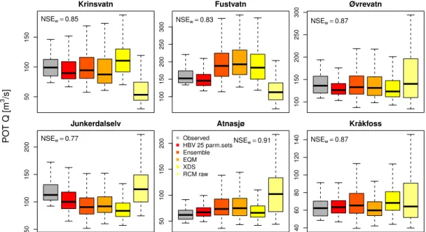
The performance of the HBV model is validated using the 25 best-fit parameter sets to estimate POT events during the reference period. These are compared with the distribution of observed POT events for the same period. In this case, the HBV simulations are based on observed meteorological data. Furthermore, we evaluated the ability of the entire en-semble (i.e. including all GCM/RCM combinations, LAMs, and hydrological parameter sets) to match the observed POT events for the reference period. A further comparison was made with HBV simulations based on the raw RCM data and the adjusted RCM data to assess the potential benefit of the adjustment procedures. The distribution of the POT events for each of these options is illustrated in Fig. 2.
The results indicate that the HBV model using the 25 best-fit parameter sets with observed climate data reproduces the observed POT events reasonably well for almost all of the catchments. For Junkerdalselv, the underestimation of the distribution of observed POT events is considerably larger than in other catchments. Junkerdalselv also has the lowest NSEw value (0.77), which is due to systematic underesti-mation of flood peaks by the calibrated model. The NSEw value for the other five catchments varies from 0.83 (Fust-vatn) to 0.91 (Atnasjø).
As expected, the absolute range and the interquartile range of the POT event distribution from the full ensemble are larger. This mainly results from the large range introduced by the locally adjusted climate projections (see the fourth and fifth box in each plot). In four catchments the quartiles match the observed distribution fairly well (Krinsvatn, Øvrevatn, Atnasjø, Kråkfoss). The largest discrepancies occur for Fust-vatn and Junkerdalselv. In both cases, the mismatch of the ensemble reflects the overestimation (Fustvatn) and underes-timation (Junkerdalselv) resulting from the different LAMs. Nevertheless, the observed distributions of POT events are always captured by the full range of the ensemble and the data locally adjusted by EQM and XDS. The performance of the ensemble in reproducing the observed POT events is the only indicator we have of how reliable the ensemble is for fu-ture projections. For Fustvatn and Junkerdalselv, this implies a lower degree of reliability as compared with the remaining catchments.
50
100
150
Krinsvatn
NSEw=0.85
100
150
200
250
300
Fustvatn
NSEw=0.83
100
150
200
250
300
Øvrevatn
NSEw=0.87
50
100
150
200
Junkerdalselv
NSEw=0.77
50
100
150
200
Atnasjø
NSEw=0.91
Observed HBV 25 parm.sets Ensemble EQM XDS RCM raw
40
60
80
100
120
140
Kråkfoss
NSEw=0.87
PO
T Q [
m
3 /s]
Figure 2.The distributions of POT events for the reference period from observed (grey) and simulated streamflow series generated by the
calibrated HBV model using (from left to right) (i) observed climate data with the 25 best-fit parameter sets, (ii) the entire ensemble (i.e. all GCM/RCM combinations, LAMs, and hydrological parameter sets), (iii) the data locally adjusted by EQM, (iv) the data locally adjusted by XDS, and (v) the raw RCM data. For the simulations (iii–v) only one best-fit HBV parameter set is considered. The NSEwvalues given
for each catchment represent the goodness of fit of the HBV model for the entire series (not only POT events) using the best parameter set identified by the calibration. Note that the ordinate’s point is not 0 and differs between the single plots.
series for Krinsvatn, Fustvatn and Atnasjø. For Fustvatn, the benefit of the local adjustment is least since the underesti-mation of the RCM raw data is only corrected to an overes-timation of almost the same magnitude and range. It is not possible to conclude which of the two LAMs is better suited for high-flow estimations, neither in general nor for specific catchments.
4.2 Changes in the temperature and precipitation regime
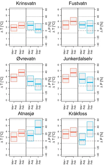
Figure 3 summarizes the interquartile ranges of the projected changes in mean temperature and precipitation sums for the spring/summer and autumn/winter seasons after local adjust-ment by EQM and XDS for the six study catchadjust-ments.
Increasing median temperatures from 2.9◦C (Krinsvatn,
spring/summer) to 4.8◦C (Øvrevatn, autumn/winter) are
pro-jected for both seasons and all catchments considered. The temperature projections indicate a larger warming in au-tumn/winter than in spring/summer in all catchments, which agrees with Engen-Skaugen et al. (2007) and Hanssen-Bauer et al. (2003, 2009). Moreover, the largest warming is found for the northernmost catchments (Øvrevatn and Junkerdal-selv) both for the spring/summer and autumn/winter periods. Generally, the results reflect findings from previous studies indicating an increasing warming signal with larger distances in latitudinal and longitudinal directions (Engen-Skaugen et al., 2007; Hanssen-Bauer et al., 2003). With the exception of
Kråkfoss, the interquartile ranges for the spring/summer sea-son are higher as compared to the autumn/winter seasea-son for all catchments.
Regarding precipitation, the medians show increasing pre-cipitation sums for both seasons and all catchments consid-ered. The increase in spring/summer precipitation tends to be larger than autumn/winter precipitation at Krinsvatn, Fust-vatn, Øvrevatn and Junkerdalselv. For Atnasjø and Kråk-foss the increase in precipitation during autumn/winter is projected to be larger than during spring and summer. The increase in autumn/winter precipitation in these two catchments is the largest projected change in precipitation (>+30 %) found within this study. Despite the positive
me-dian values, the ensemble does not consistently show positive changes in the projections. The first quartile for the changes in autumn/winter precipitation indicates decreasing precipi-tation sums for Krinsvatn, Fustvatn, Øvrevatn and Junkerdal-selv. For Atnasjø and Kråkfoss the first quartile of the dis-tribution indicates decreasing spring/summer precipitation sums. Generally, the results for these six catchments corre-spond to the regional differences in seasonal precipitation change previously presented in Hanssen-Bauer et al. (2009).
4.3 Changes in flood seasonality
Mar − A ug S ep − F eb 0 1 2 3 4 5 6 ∆ T K[ °C] Mar − A ug S ep − F eb − 40 − 20 0 20 40 60 ∆ P K[ i]
Atnasjø
Mar − A ug S ep − F eb 0 1 2 3 4 5 6 ∆ T K[ °C] Mar − A ug S ep − F eb − 40 − 20 0 20 40 60 ∆ P K[ i]Kråkfoss
Mar − A ug S ep − F eb 0 1 2 3 4 5 6 ∆ T K[ °C] Mar − A ug S ep − F eb − 40 − 20 0 20 40 60 ∆ P K[ i]Krinsvatn
Mar − A ug S ep − F eb 0 1 2 3 4 5 6 ∆ T K[ °C] Mar − A ug S ep − F eb − 40 − 20 0 20 40 60 ∆ P K[ i]Fustvatn
Mar − A ug S ep − F eb 0 1 2 3 4 5 6 ∆ T K[ °C] Mar − A ug S ep − F eb − 40 − 20 0 20 40 60 ∆ P K[ i]Junkerdalselv
Mar − A ug S ep − F eb 0 1 2 3 4 5 6 ∆ T K[ °C] Mar − A ug S ep − F eb − 40 − 20 0 20 40 60 ∆ P K[ i]Øvrevatn
Figure 3.The interquartile ranges of the projected changes from the
reference (1961–1990) to the future period (2071–2099) in mean temperature (left panel) and precipitation sums (right panel) for the spring/summer and autumn/winter seasons as they are locally ad-justed by EQM and XDS for the six study catchments.
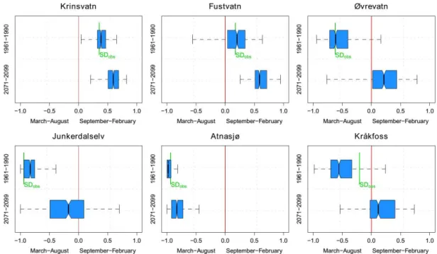
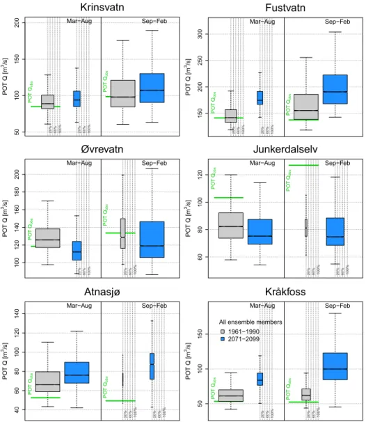
For the reference period, the SD quartiles for the coastal catchments Krinsvatn and Fustvatn show positive values, indicating a dominance of autumn/winter POT events un-der the current climate. For Øvrevatn and Junkerdalselv in the north, as well as for Atnasjø and Kråkfoss in central and south-eastern Norway, the SD quartiles indicate domi-nant POT events during spring/summer. The dominance of spring/summer events is largest for Atnasjø, but Junkerdal-selv also shows a distinct spring/summer pattern with neg-ative SD values for all ensemble realizations. For Kråkfoss, this dominance is least pronounced. The observed flood sea-sonality (indicated by the green bars) is matched reason-ably well in five of the six catchments (Krinsvatn, Fustvatn, Øvrevatn, Junkerdalselv, Atnasjø), with Fustvatn and Øvre-vatn having the best matches. For Kråkfoss, however, the
SD values for the majority of the ensemble realizations are
rather low suggesting that the dominance of spring/summer events is exaggerated to some degree by the model simu-lations. Simulated SD values based on observed meteoro-logical input data and the 25 best-fit parameter sets were, however, found to be very similar to the SD value based on observed runoff (not shown). Thus, the overestimation of spring/summer events at Kråkfoss is a consequence of cli-mate input data, rather than the hydrological modelling.
For the future period, theSDvalues are higher for all catch-ments. That means that the importance of autumn/winter events is projected to increase in all catchments considered. The lowest impact is found for Atnasjø where the domi-nance of spring/summer events persists into the future. How-ever, for Øvrevatn and Kråkfoss considerably higherSD val-ues indicate a possible seasonal shift in the flood regimes sinceSD becomes positive for almost the entire
interquar-tile of all ensemble realizations. Changes towards dominant autumn/winter events are also indicated for some ensemble members for Junkerdalselv. However, the first and second quartiles still show negativeSDvalues.
The ranges in the projections given by the boxplots illus-trate the uncertainty associated with the ensemble. For the reference period, this is highest for Fustvatn and Kråkfoss. For the future period, the highest ranges are found for Øvre-vatn, Junkerdalselv and Kråkfoss, which show the largest change in flood seasonality. Note that the projected changes in seasonality are significant (with 95 % confidence) for all catchments, as none of the notches of the boxplots for the reference and future periods are overlapping.
4.4 Changes in the magnitude vs. the frequency of events
After having detected changes in flood seasonality, the ques-tion arises as to whether these result from changes in flood magnitude vs. frequency in the two respective seasons. Fig-ure 5 summarizes the POT events for all ensemble realiza-tions according to their associated magnitudes and number of occurrences for the two seasons.
For the coastal catchments, Krinsvatn and Fustvatn, Fig. 5 shows that both the relative number and the magnitude of POT events increase in autumn/winter during the future pe-riod. For spring/summer the magnitude also increases but the frequency decreases (i.e. the blue boxes show smaller widths). Together, this explains the intensification of the sea-sonality index SD towards autumn/winter events. The
indi-Figure 4.Boxplots showing the seasonality indexSDfor all ensemble realizations for the reference and future periods. The boxes show the interquartile of the values; the whiskers show the full range of the projections. The green bars in the upper panel of each plot (SDobs) indicate
the observed seasonality indexSD.
cates that spring/summer events are very dominant in both the current and future climates. Figure 5 establishes that this dominance reflects the frequency of the events in the POT series, and not necessarily the magnitude. Future flood magnitudes increase slightly for both seasons, while fre-quencies increase particularly in the autumn/winter period. This is responsible for the slight shift in seasonal index in Fig. 4. Finally, Fig. 5 also illustrates that the large seasonal shift for Kråkfoss is caused by both frequencies (decrease in spring/summer, increase in autumn/winter) and magnitudes. Future flood magnitudes increase in both seasons, but the in-crease in autumn/winter is considerably larger.
Note that the discrepancies between the observed and sim-ulated POT magnitudes for the reference period (i.e. Fig. 2) are also reflected in the seasonal values in Fig. 5. The large discrepancy at Junkerdalselv (underestimation) and Atnasjø (overestimation) for the autumn/winter period is due to the limited number of observed events during these months. The correspondence between the observed and simulated sea-sonal median POT event magnitudes at Kråkfoss is compara-tively better than for the seasonality indexSD(Fig. 4). Since the distribution of the POT event magnitudes are very similar both for the spring/summer and the autumn/winter seasons, the bias ofSDtowards spring/summer results from an
over-estimation of the event frequency for this season.
The median changes in the POT event magnitudes from the references to the future period are significant (with 95 % con-fidence) for all catchments, as none of the illustrated notches for the respective period is overlapping.
4.5 Changes in FGPs
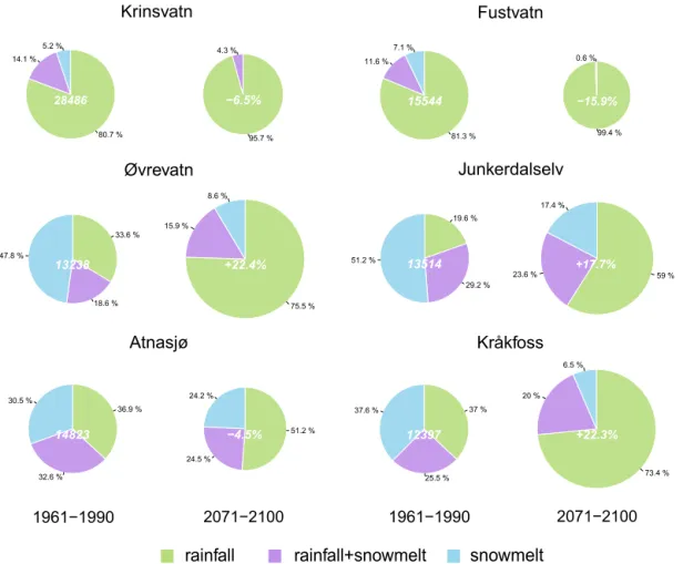
In the previous sections, we established that autumn/winter events will become more dominant in the future. This is consistent over all investigated catchments, although there are differences with respect to their underlying causes (i.e. changes in frequency, magnitude, or both). In gen-eral, we would expect that an increasing dominance of au-tumn/winter events corresponds to an increasing importance of rainfall as a FGP. Figure 6 shows how the percentage of different flood generating processes will change between the reference and the future periods.
20ø 60ø 100ø 20ø 60ø 100ø
P
O
T
Qobs PO
T
Qobs
Mar−Aug Sep−Feb
50
100
150
200
P
O
T
kQ
k[
m
37s]
Krinsvatn
20ø 60ø 100ø 20ø 60ø 100ø
P
O
T
Qobs
P
O
T
Qobs
Mar−Aug Sep−Feb
150
200
250
300
P
O
T
kQ
k[
m
37s]
Fustvatn
20ø 60ø 100ø 20ø 60ø 100ø
P
O
T
Qobs P
O
T
Qobs
Mar−Aug Sep−Feb
100
120
140
160
180
200
P
O
T
kQ
k[
m
37s]
Øvrevatn
20ø 60ø 100ø 20ø 60ø 100ø
P
O
T
Qobs
P
O
T
Qobs
Mar−Aug Sep−Feb
60
80
100
120
P
O
T
kQ
k[
m
37s]
Junkerdalselv
20ø 60ø 100ø 20ø 60ø 100ø
P
O
T
Qobs
P
O
T
Qobs
Mar−Aug Sep−Feb
40
60
80
100
120
140
P
O
T
kQ
k[
m
37s]
Atnasjø
20ø 60ø 100ø 20ø 60ø 100ø
P
O
T
Qobs
P
O
T
Qobs
Mar−Aug Sep−Feb
50
100
150
P
O
T
kQ
k[
m
37s]
Kråkfoss
Allkensemblekmembers 1961−1990 2071−2099
Figure 5.Boxplots showing the median and interquartile magnitudes of the simulated POT events from all ensemble realizations for the
reference (grey boxes) and future periods (blue boxes), separated with respect to the two basic flood seasons in Norway (spring/summer – left panels; autumn/winter – right panels). The whisker range corresponds to twice the interquartile range. The green bars (POTobs) indicate
the median magnitudes of observed POT events. The width of the boxes illustrates the seasonal distribution in the frequency of the POT events: Per catchment and period, the smaller boxes are scaled compared to the larger boxes representing the dominant flood season in terms of flood frequency.
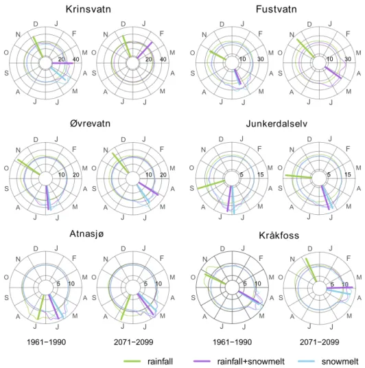
Figure 7 shows the circular kernel density functions of the events for each FGP and illustrates the relationship between the changes in the FGPs and the median magnitude of the events as a function of their mean Julian date of occurrence.
Snowmelt-associated events are connected with an earlier timing and POT events of a decreased magnitude in catch-ments where this FGP continues to be relevant in the gen-eration of high flows. Higher mean temperatures in the fu-ture period (Fig. 3) lead to an earlier onset of the annual snowmelt season. For the catchments which continue to have peak discharges derived from snowmelt in the future period, the circular mean Julian dates of occurrence of the snowmelt-generated events is estimated to be 14–26 days earlier
80.785 14.185
5.285
28486
95.785 4.385
Krinsvatn
−6.5%
81.385 11.685
7.185
15544
99.485 0.685
Fustvatn
−15.9%
33.685
18.685 47.885
13238
75.585 15.985
8.685
Øvrevatn
+22.4%
19.685
29.285 51.285 13514
5985 23.685
17.485
Junkerdalselv
+17.7%
36.985
32.685 30.585
14823 51.285
24.585 24.285
Atnasjø
−4.5%
3785
25.585 37.685
12397
73.485 2085
6.585
Kråkfoss
+22.3%
rainfall rainfall+snowmelt
snowmelt
1961−1990 2071−2100 1961−1990 2071−2100
Figure 6.Percentage of POT events according to their FGPs in relation to the total number of events for the reference (left pie charts)
and future periods (right pie charts) derived by all ensemble realizations. The diameter of the pie charts for the future period indicates the direction of change in the total number of events. Total numbers of events for the reference period and the percentage of change in the number of events for the future period are given by the white numbers within the pie charts.
and warmer winters in the future period (Vikhamar Schuler et al., 2006).
Rainfall-generated events tend to occur later within the year across all catchments. The later mean timing of rainfall-generated events highlights the increasing importance of winter rainfall floods in the future period. This corresponds to projected changes in the temperature and precipitation regimes (Fig. 3), which lead to a shorter snow season and reduced snow storage, and to an increasing relevance of episodes with intermittent rainfall and winter snowmelt due to higher winter temperatures (Hanssen-Bauer et al., 2009). For Øvrevatn, Junkerdalselv and Kråkfoss, this suggests that winter precipitation is no longer primarily received as snow-fall such that the contribution of snowmelt to runoff is considerably less in the future period. Thus, the strongest changes in flood seasonality are observed for these three catchments which is in line with Arnell (1999), who con-cludes that the most significant changes in flow regimes oc-cur where snowfall becomes less important due to higher temperatures. The effects of increased evaporation during late summer due to higher temperatures may also amplify the
later mean timing of rainfall-generated events, as soil mois-ture deficits may have a more pronounced role in attenuating heavy rainfalls during the autumn period.
The mean magnitudes of rainfall-generated events are pro-jected to increase at Fustvatn, Atnasjø and Kråkfoss which explains the increasing POT-event magnitudes during au-tumn and winter in these catchments as shown in Fig. 5. The increasing magnitudes of autumn/winter events at Krins-vatn (Fig. 5) result from an earlier circular mean timing of the rainfall+snowmelt-generated events in the future period
Kråkfoss Atnasjø Junkerdalselv Øvrevatn Fustvatn Krinsvatn
1961−1990 2071−2099
5 10 5 10
5 10 5 10
5 15 5 15
J F M A M J J A S O N D J F M A M J J A S O N D
10 20 10 20
J F M A M J J A S O N D J F M A M J J A S O N D
10 30 10 30
J F M A M J J A S O N D J F M A M J J A S O N D
20 40 20 40
J F M A M J J A S O N D J F M A M J J A S O N D
1961−1990 2071−2099
rainfall rainfall+snowmelt snowmelt
J F M A M J J A S O N D J F M A M J J A S O N D J F M A M J J A S O N D J F M A M J J A S O N D
Figure 7.Circular plots showing (i) the circular kernel density function of the simulated POT events according to their FGPs (normalized;
no units), and (ii) the median POT-event magnitude (mm day−1) as bars according to their circular mean Julian date of occurrence and their
FGPs for the reference and future periods.
The results also illustrate that changes in flood seasonality cannot be directly inferred from seasonal changes in precip-itation and temperature. Hydrological modelling is required to highlight the changing role of snow storage and its effect on flood generation.
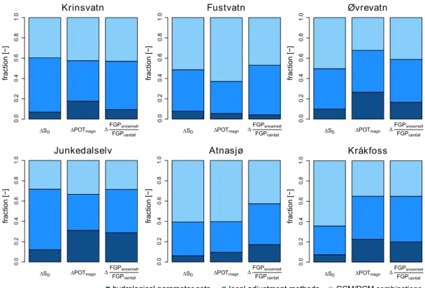
4.6 Contribution of ensemble components to uncertainty
Figure 8 shows the fractional variance from the different sources of the ensemble as they contribute to the total vari-ance regarding the changes in the indexSD, the POT
magni-tudes and the FGPs presented in Figs. 4–7.
First of all, the GCM/RCM combinations and the LAMs are the dominant sources of uncertainty for all catchments and variables considered. Hydrological model parameteri-zation tends to be the smallest contributor to overall un-certainty, which is in line with earlier studies (e.g. Wilby and Harris, 2006; Kay et al., 2008; Prudhomme and Davies, 2008; Dobler et al., 2012b). Note, however, that there are ex-ceptions where the variance due to the hydrological model
parameterization is as high as that due to the LAMs or the climate projections (i.e. Junkerdalselv, second and third columns). Focusing on the target variables, hydrological pa-rameter uncertainty tends to be less important for changes in the seasonality indexSDas compared with changes in the POT-event magnitudes and the dominant FGPs.
Kråkfoss
fr
act
ionw
[
−
]
hR
h
hR
p
hR
4
hR
6
hR
8
yR
h
∆SD ∆POTmagn ∆
FGPsnowmelt
FGPrainfall
Atnasjø
fr
act
ionw
[
−
]
hR
h
hR
p
hR
4
hR
6
hR
8
yR
h
∆SD ∆POTmagn ∆
FGPsnowmelt
FGPrainfall
Junkedalselv
fr
act
ionw
[
−
]
hR
h
hR
p
hR
4
hR
6
hR
8
yR
h
∆SD ∆POTmagn ∆
FGPsnowmelt
FGPrainfall
Øvrevatn
fr
act
ionw
[
−
]
hR
h
hR
p
hR
4
hR
6
hR
8
yR
h
∆SD ∆POTmagn ∆
FGPsnowmelt
FGPrainfall
Fustvatn
fr
act
ionw
[
−
]
∆SD ∆POTmagn ∆
FGPsnowmelt
FGPrainfall
Krinsvatn
fr
act
ionw
[
−
]
hR
h
hR
p
hR
4
hR
6
hR
8
yR
h
∆SD ∆POTmagn ∆
FGPsnowmelt
FGPrainfall
hR
h
hR
p
hR
4
hR
6
hR
8
yR
h
GCMbRCMwcombinations localwadjustmentwmethods
hydrologicalwparameterwsets
Figure 8.The fractions of total variance (–) as a measure for uncertainty, explained by (i) the GCM/RCM combinations (light blue), (ii) the
local adjustment methods (medium blue), and (iii) the hydrological parameterization (dark blue) with respect to three target variables: (1) change in the seasonality indexSD, (2) change in the mean POT event magnitude, and (3) change in the ratio of snowmelt- and
rainfall-generated POT events.
2013; Merz et al., 2011). The choice of the reference period (1961(1966)–1990) may imply that we have detected quite stable parameters for that period since the pronounced warm-ing durwarm-ing the recent years are not included in the calibra-tion. These parameters, however, may be even less represen-tative for the future conditions. Merz et al. (2011) have cal-ibrated a similar version of the HBV model for six consec-utive 5-year periods for a comprehensive set of catchments in Austria. They found notable time trends in the calibrated parameters representing snow dynamics and soil moisture processes which lead to considerable biases especially in high flows. For our results, that implies that the hydrologi-cal model parameter uncertainty limits the reliability of the estimated changes in the proportion of rainfall and snowmelt and their effects on flood seasonality and FGPs.
One option for dealing with that issue are differential split sample tests (Klemeš, 1986). These are usually used to evaluate parameter sets which are optimized for contrast-ing conditions. Seibert (2003) calibrated the HBV model in four Swedish catchments on years with lower runoff peaks and tested the calibrated parameters for years with higher peaks, finding a decrease in model performance. Coron et al. (2012) introduced generalized split-sample tests, which systematically test all possible combinations of calibration-validation periods using a 10-year moving window over the
observation time period. They also pointed out a lack of robustness in hydrological model parameters tested in cli-mate conditions which differ to those used for model cal-ibration. Similar schemes need to be adapted for seasonal-ity purposes, i.e. identifying contrasting periods in terms of seasonal flood prevalence and dominant FGPs. Differential split sample testing can then indicate parameter robustness when applied under contrasting seasonality conditions. They may also indicate parameter sets which are suitable for runoff simulations under future conditions. This approach, however, presupposes that relevant changes can already be detected in the observation data and that contrasting periods are long enough for a sufficient model calibration.
5 Conclusions
The results indicate that the HBV model, including the use of 25 best-fit parameter sets, is able to reproduce ob-served distributions of flood events reasonably well for five out of six study catchments for the reference period. Small discrepancies between the event distributions simulated by the locally adjusted climate projection data and the observed event distributions slightly reduce the reliability of the en-semble setup for two catchments (Fustvatn, Junkerdalselv). For the remaining four catchments the ensemble reproduces the observed flood-event distributions fairly well. The benefit of post-processing the RCM raw data has also been demon-strated. However, no distinct ranking emerged regarding the performance of the two LAMs applied.
Reconsidering our research questions, the following con-clusions can be drawn:
– How might the existing patterns of flood seasonality
change under a future climate? Autumn/winter floods
become more important in all the catchments con-sidered. For the two coastal catchments that suggests an intensification of the current autumn/winter flood regime. For the high-mountain catchment, Atnasjø, in central Norway, the dominance of spring/summer floods will be slightly reduced. For the northernmost catchments, Øvrevatn and Junkerdalselv, as well as for the south-eastern catchment, Kråkfoss, the increase in autumn/winter floods is largest and may lead to a systematical shift in the current flood regimes from spring/summer to autumn/winter.
– How are the shifts in seasonality related to changes in
the magnitude vs. changes in the frequency of events?
Changes in flood seasonality from spring/summer to-wards autumn/winter are the result of increasing event magnitudes or frequencies, or a combination of both, during the autumn and winter months. Changes in seasonal frequency, however, are more relevant than changes in seasonal magnitude since two of the catch-ments with the strongest changes in flood seasonal-ity (Øvrevatn and Junkerdalselv) show decreasing flood magnitudes but large shifts in the seasonal frequency of events.
– Are changes in flood seasonality associated with
changes in the FGPs? The change towards more
au-tumn/winter events corresponds to an increasing rele-vance of rainfall as a FGP. Rainfall becomes more dom-inant where it has already been domdom-inant and it re-places snowmelt as the dominant FGP in the remaining catchments. The largest increases in the relative role of rainfall correspond with the largest shifts in flood sea-sonality (Øvrevatn, Junkerdalselv, Kråkfoss). In these catchments, less snow accumulation and shorter snow seasons due to increased winter temperatures lead to a considerable decrease in the frequency and magnitude of snowmelt-generated events. Additionally,
rainfall-generated events occur more often and also later within the autumn/winter period. Thus, the largest changes in the FGPs are closely connected with temperature effects which determine the relative role of snowmelt vs. rain-fall. This has a major influence on the seasonal distribu-tion of floods.
– What is the relative importance of the different ensemble
components in contributing to the overall variance as a measure of the uncertainty in the projected changes?
For changes in flood seasonality the ensemble range is largest in those catchments for which the largest sea-sonal changes are projected. The climate projections (i.e. the GCM/RCM combinations) or the LAMs tend to be the largest contributor to the total variance. How-ever, the relative role of the hydrological model pa-rameterization compared to the other two contributors is highest for those catchments showing the most pro-nounced seasonal changes. This is consistent with an earlier study of climate change impacts in four Norwe-gian catchments (Lawrence and Haddeland, 2011), and confirms the lack of robustness in HBV parameteriza-tions for simulaparameteriza-tions with transient hydroclimatological conditions which lead to changes in the flood regime. It further stresses the need for alternative calibration ap-proaches which improve the transferability of hydrolog-ical model parameters under non-stationary conditions. Although the catchments analysed within this study rep-resent a large variety of climate conditions in Norway, the sample size is too small to allow for robust regional conclu-sions on changes in the seasonality and generation processes of floods. The results presented here can only indicate pos-sible responses to climate change in terms of flood season-ality and FGPs for catchments with similar hydroclimato-logical regimes and physical conditions. For robust regional conclusions, the proposed methodology needs to be applied for a larger sample of catchments. Alternatively, a grid-based modelling approach covering the whole country could also be used, although such results must be interpreted with care in areas lacking data for model calibration.
Acknowledgements. The first author acknowledges the Helmoltz graduate research school GeoSim for funding the PhD studentship and NVE for funding study visits to Norway. The second author acknowledges support from NVE for the internally funded project Climate change and future floods. The regional climate model simulations stem from the EU FP6 project ENSEMBLES, whose support is gratefully acknowledged. Gerd Bürger (University of Potsdam) is thanked for his great support on downscaling the RCM data by XDS. The Potsdam Graduate School (PoGS) is acknowledged for supporting the service charge cover for this open access publication. Daniel Viviroli and two anonymous referees are thanked for their comments on an earlier version of this manuscript.
References
Andréasson, J. and Bergström, S.: Hydrological change-climate change impact simulations for Sweden, AMBIO A J. Hum. Env-iron., 33, 228–234, doi:10.1579/0044-7447-33.4.228, 2004. Arnell, N. W.: The effect of climate change on hydrological regimes
in Europe: a continental perspective, Global Environ. Change, 9, 5–23, doi:10.1016/S0959-3780(98)00015-6, 1999.
Bayliss, A. C. and Jones, R. C.: Peaks-Over-Threshold Flood Database: Summary Statistics and Seasonality, Wallingford, UK, 1993.
Beldring, S., Engen-Skaugen, T., Førland, E. J., and Roald, L. A.: Climate change impacts on hydrological processes in Norway based on two methods for transferring regional climate model results to meteorological station sites, Tellus A, 60, 439–450, doi:10.1111/j.1600-0870.2008.00306.x, 2008.
Benestad, R. E.: Association between trends in daily rainfall per-centiles and the global mean temperature, J. Geophys. Res.-Atmos., 118, 10802–10810, doi:10.1002/jgrd.50814, 2013. Beniston, M., Stephenson, D. B., Christensen, O. B., Ferro, C. A.
T., Frei, C., Goyette, S., Halsnaes, K., Holt, T., Jylhä, K., Koffi, B., Palutikof, J., Schöll, R., Semmler, T., and Woth, K.: Fu-ture extreme events in European climate: an exploration of re-gional climate model projections, Climatic Change, 81, 71–95, doi:10.1007/s10584-006-9226-z, 2007.
Bergström, S.: Development and application of a conceptual runoff model for Scandinavian catchments, Report No. 7 RHO, Swedish Meteorological and Hydrological Institute – SMHI, Nörrköping, 1976.
Bergström, S.: The HBV model, in: Computer Models of Water-shed Hydrology, edited by: Singh, V. P., Water Resources Publi-cations, Highlands Ranch, CO, 443–476, 1995.
Bhend, J. and von Storch, H.: Consistency of observed winter pre-cipitation trends in northern Europe with regional climate change projections, Clim. Dynam., 31, 17–28, doi:10.1007/s00382-007-0335-9, 2007.
Blöschl, G., Viglione, A., Merz, R., Parajka, J., Salinas, J. L., and Schöner, W.: Auswirkungen des Klimawandels auf Hochwasser und Niederwasser, Österreichische Wasser- und Ab-fallwirtschaft, 63, 21–30, doi:10.1007/s00506-010-0269-z, 2011. Boé, J., Terray, L., Habets, F., and Martin, E.: Statistical and dynamical downscaling of the Seine basin climate for hydro-meteorological studies, Int. J. Climatol., 27, 1643–1655, doi:10.1002/joc.1602, 2007.
Brigode, P., Oudin, L., and Perrin, C.: Hydrological model parame-ter instability: A source of additional uncertainty in estimating the hydrological impacts of climate change?, J. Hydrol., 476, 410–425, doi:10.1016/j.jhydrol.2012.11.012, 2013.
Bronstert, A., Kolokotronis, V., Schwandt, D., and Straub, H.: Com-parison and evaluation of regional climate scenarios for hydro-logical impact analysis?: General scheme and application exam-ple, Int. J. Climatol., 1594, 1579–1594, doi:10.1002/joc.1621, 2007.
Bürger, G.: Expanded downscaling for generating local weather scenarios, Clim. Res., 7, 111–128, doi:10.3354/cr007111, 1996. Bürger, G., Reusser, D., and Kneis, D.: Early flood warnings from empirical (expanded) downscaling of the full ECMWF En-semble Prediction System, Water Resour. Res., 45, W10443, doi:10.1029/2009WR007779, 2009.
Burn, D. H.: Catchment similarity for regional flood frequency analysis using seasonality measures, J. Hydrol., 202, 212–230, doi:10.1016/S0022-1694(97)00068-1, 1997.
Chen, J., Brissette, F. P., and Leconte, R.: Uncertainty of downscaling method in quantifying the impact of cli-mate change on hydrology, J. Hydrol., 401, 190–202, doi:10.1016/j.jhydrol.2011.02.020, 2011.
Coron, L., Andréassian, V., Perrin, C., Lerat, J., Vaze, J., Bourqui, M., and Hendrickx, F.: Crash testing hydrological models in contrasted climate conditions: An experiment on 216 Australian catchments, Water Resour. Res., 48, W05552, doi:10.1029/2011WR011721, 2012.
Déqué, M., Rowell, D. P., Lüthi, D., Giorgi, F., Christensen, J. H., Rockel, B., Jacob, D., Kjellström, E., Castro, M., and Hurk, B.: An intercomparison of regional climate simulations for Europe: assessing uncertainties in model projections, Climatic Change, 81, 53–70, doi:10.1007/s10584-006-9228-x, 2007.
Déqué, M., Somot, S., Sanchez-Gomez, E., Goodess, C. M., Jacob, D., Lenderink, G., and Christensen, O. B.: The spread amongst ENSEMBLES regional scenarios: regional climate models, driv-ing general circulation models and interannual variability, Clim. Dynam., 38, 951–964, doi:10.1007/s00382-011-1053-x, 2011. Déry, S. J., Stahl, K., Moore, R. D., Whitfield, P. H., Menounos, B.,
and Burford, J. E.: Detection of runoff timing changes in pluvial, nival, and glacial rivers of western Canada, Water Resour. Res., 45, W04426, doi:10.1029/2008WR006975, 2009.
Dobler, C., Bürger, G., and Stötter, J.: Assessment of climate change impacts on flood hazard potential in the Alpine Lech watershed, J. Hydrol., 460–461, 29–39, doi:10.1016/j.jhydrol.2012.06.027, 2012a.
Dobler, C., Hagemann, S., Wilby, R. L., and Stötter, J.: Quantify-ing different sources of uncertainty in hydrological projections in an Alpine watershed, Hydrol. Earth Syst. Sci., 16, 4343–4360, doi:10.5194/hess-16-4343-2012, 2012b.
Dobler, C., Bürger, G., and Stötter, J.: Simulating future precipita-tion extremes in a complex Alpine catchment, Nat. Hazards Earth Syst. Sci., 13, 263–277, doi:10.5194/nhess-13-263-2013, 2013. Dyrrdal, A. V., Isaksen, K., Hygen, H., and Meyer, N.: Changes in
meteorological variables that can trigger natural hazards in Nor-way, Clim. Res., 55, 153–165, doi:10.3354/cr01125, 2012. Dyrrdal, A. V., Saloranta, T., Skaugen, T., and Stranden, H. B.:
Changes in snow depth in Norway during the period 1961–2010, Hydrol. Res., 44, 169, 169–179, doi:10.2166/nh.2012.064, 2013. Engen-Skaugen, T., Haugen, J. E., and Tveito, O. E.: Temperature scenarios for Norway: from regional to local scale, Clim. Dy-nam., 29, 441–453, doi:10.1007/s00382-007-0241-1, 2007. Fleig, A. K., Andreassen, L. M., Barfod, E., Haga, J., Haugen, L.
E., Hisdal, H., Melvold, K., and Saloranta, T.: Norwegian Hy-drological Reference Dataset for Climate Change Studies, Re-port No. 2, Norwegian Water Resources and Energy Directorate – NVE, Oslo, 2013.
Fowler, H. J. and Ekström, M.: Multi-model ensemble estimates of climate change impacts on UK seasonal precipitation extremes, Int. J. Climatol., 29, 385–416, doi:10.1002/joc.1827, 2009. Fowler, H. J., Blenkinsop, S., and Tebaldi, C.: Linking climate