D. Lawrence1, E. Paquet2, J. Gailhard2, and A. K. Fleig1
1Norwegian Water Resources and Energy Directorate (NVE), Oslo, Norway 2Electricité de France (EDF-DTG), Grenoble, France
Correspondence to:D. Lawrence (dela@nve.no)
Received: 28 September 2013 – Published in Nat. Hazards Earth Syst. Sci. Discuss.: 26 November 2013 Revised: 11 April 2014 – Accepted: 11 April 2014 – Published: 23 May 2014
Abstract.Simulation methods for extreme flood estimation represent an important complement to statistical flood fre-quency analysis because a spectrum of catchment conditions potentially leading to extreme flows can be assessed. In this paper, stochastic, semi-continuous simulation is used to es-timate extreme floods in three catchments located in Nor-way, all of which are characterised by flood regimes in which snowmelt often has a significant role. The simulations are based on SCHADEX, which couples a precipitation prob-abilistic model with a hydrological simulation such that an exhaustive set of catchment conditions and responses is sim-ulated. The precipitation probabilistic model is conditioned by regional weather patterns, and a bottom–up classifica-tion procedure was used to define a set of weather patterns producing extreme precipitation in Norway. SCHADEX es-timates for the 1000-year (Q1000) discharge are compared with those of several standard methods, including event-based and long-term simulations which use a single extreme precipitation sequence as input to a hydrological model, sta-tistical flood frequency analysis based on the annual max-imum series, and the GRADEX method. The comparison suggests that the combination of a precipitation probabilistic model with a long-term simulation of catchment conditions, including snowmelt, produces estimates for given return pe-riods which are more in line with those based on statistical flood frequency analysis, as compared with the standard sim-ulation methods, in two of the catchments. In the third case, the SCHADEX method gives higher estimates than statis-tical flood frequency analysis and further suggests that the seasonality of the most likely Q1000 events differs from that of the annual maximum flows. The semi-continuous stochastic simulation method highlights the importance of
considering the joint probability of extreme precipitation, snowmelt rates and catchment saturation states when as-signing return periods to floods estimated by precipitation-runoff methods. The SCHADEX methodology, as applied here, is dependent on observed discharge data for calibra-tion of a hydrological model, and further study to extend its application to ungauged catchments would significantly enhance its versatility.
1 Introduction
Precipitation-runoff methods have a long history of applica-tion in design flood analyses and represent an important com-plement to statistical methods, particularly for estimating floods with long return periods. Although event-based meth-ods continue to dominate design flood analysis in practice in many countries, long-term simulation methods are now also feasible due both to increased computational capacity and to advances in the methodologies for generating rainfall input to the simulation (e.g. see discussions in Boughton and Droop, 2003 and Pathiraja et al., 2012). In particular, the in-troduction and further development of continuous simulation methods for generating a synthetic time series of long dura-tion which can then also be analysed using statistical flood frequency analysis (e.g. Cameron et al., 1999; Blazkova and Beven, 2004) have highlighted the added benefits of such an approach.
superimposed on a hydrological simulation based on a histor-ical period. The SCHADEX “semi-continuous” simulation method (Paquet et al., 2006, 2013) is such an approach and represents an efficient strategy for focusing on flood gener-ating events within a simulation framework. In addition, de-sign flood analyses for dam safety in Finland (see Veijalainen and Vehviläinen, 2008, for a brief summary) and Sweden (see Bergström, et al., 1992, 2008) also employ hydrologi-cal simulations run over a 10- to 40-year historihydrologi-cal period coupled with a hypothetical design precipitation sequence, such that a range of potential catchment responses to ex-treme precipitation are sampled. In this work, we therefore make a distinction between (1) event-based methods which model the catchment response to a selected input precipita-tion sequence and generally assume a set of pre-event condi-tions for the catchment; and (2) long-term simulation meth-ods which couple a hydrological simulation for characteris-ing varycharacteris-ing catchment conditions with an input precipitation, based either on a single design precipitation sequence or on a probabilistic methodology for generating multiple precipi-tation events. This is in contrast to the distinction that is typ-ically used for describing precipitation-runoff methods for design flood analysis, i.e. event-based vs. continuous simu-lation methods (e.g. Grimaldi et al., 2013). A further distinc-tion could be made between methods which use a fixed de-sign precipitation sequence and those which consider a range of possible rainfall events. Flood simulations using a sin-gle design hyetograph assume a fixed relationship between the return period of rainfall event and that of the simulated flood event, which is itself problematic (Rahman et al., 2002; Kuczera et al., 2006). In such simulations, the temporal se-quence of the rainfall is also specified in terms of the shape of the hyetograph and the duration of the event. Alternative methods which consider catchment response to a range of precipitation events, either as an event-based model or in a long-term simulation mode, have clear advantages over the classical use of a design hyetograph with respect to assign-ing return periods to the simulated events (Cameron et al., 1999; Paquet et al., 2013).
From the perspective of the practitioner, it is important that extreme flood analysis methods, regardless of the approach used, produce consistent estimates which are comparable be-tween applications in differing regions and, simultaneously, that the methods are not severely restricted by their data re-quirements. In the Nordic countries snowmelt is an impor-tant factor contributing to flood generation in most areas, and the selected modelling methodology must include a robust strategy for accounting for this contribution to peak runoff. This can be a particular challenge for event-based methods, especially in areas and for seasons for which snow accu-mulation and melting are quite transient (e.g. early autumn in mountainous areas or mid-winter in some coastal areas) or spatially varying (e.g. in catchments with pronounced to-pography). Long-term simulation methods are, in principle, more suitable for estimating the return period of combined
snowmelt/rainfall events as variability in the snowmelt con-tribution to runoff, as well as in the saturation status of the catchment, are to a certain degree simulated by the hydro-logical model. Although recent publications (e.g. Camici et al., 2011; Pathiraja et al. 2012) have highlighted the advan-tages of long-term simulation with respect to accounting for varying antecedent soil moisture conditions, little published work has evaluated its use for extreme flood estimation in ar-eas where snowmelt can have a significant role throughout much of the year.
In this work, we consider extreme flood estimation in three catchments of moderate size (207–436 km2), all
lo-cated in Norway. The three catchments are susceptible to ex-treme flows caused by a combination of heavy rainfall and snowmelt, although there are differences in the seasonality of peak flows and in the relative contribution of snowmelt to annual runoff. The focus here is on the application of SCHADEX semi-continuous simulation and particularly considers its suitability for analysing extreme floods caused by a combination of extreme precipitation and snowmelt. The results of the SCHADEX application are compared with other methods for design flood analysis in the Nordic region, including (1) a simple, event-based, method for estimating peak discharge in response to a predefined extreme precipita-tion sequence, which represents standard practice for design flood analysis in Norway; and (2) a long-term simulation us-ing a calibrated hydrological model together with an extreme precipitation sequence that is iterated through a simulation period, which is similar to the simulation methods used for design flood analyses in Finland and Sweden. A comparison of all three precipitation-runoff methods is also made with statistical flood frequency analysis based on observed dis-charge data and with the GRADEX method (Guillot, 1993) for flood estimation, which is widely applied outside of the Nordic region.
2 Study catchments
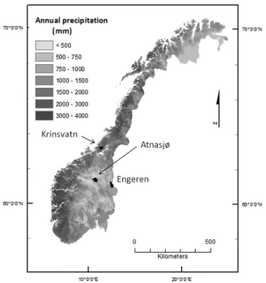
Three catchments were used for the SCHADEX applica-tions and the comparisons with other methods: (1) Atnasjø (463 km2), located in the central mountainous region of
southern Norway, (2) Engeren (395 km2), located in the in-land region of eastern Norway, and (3) Krinsvatn (207 km2), located along the western coast of mid-Norway (Fig. 1). These particular catchments were selected as they all have (a) long daily discharge records, i.e. approximately 100 years of record; (b) available hourly discharge values for up to twenty-year periods which can be used for developing es-timates of peak to volume ratios for the SCHADEX method; (c) extreme flood regimes characterised by a combination of heavy rainfall and snowmelt; and (d) relatively pristine catch-ments largely unaffected by river regulation.
Forest (%) 21 49 21
Lake (%) 2 4 8
Marsh and bog (%) 3 16 10
Sparse vegetation over treeline (%) 70 30 61 Other (e.g. meadows, populated areas) (%) 4 0 1 Effective lake percentage (%) 1.1 2.7 1.1 Hydrologic regime
Mean annual runoff (mm yr−1) 655 588 1917
Mean annual maximum daily flow (m3s−1) 71 53 131
Maximum observed daily discharge (m3s−1) 187 136 336
Season for annual maximum flows Mid-May– May– September– early July mid-June February
snowmelt-dominated flood regime, with the highest annual flows usually occurring in late May and June. High flows can, however, also occur in the late summer and early au-tumn in response to heavy precipitation, and sometimes in conjunction with early autumn snow accumulation and melt-ing. The mean annual flood for the period 1916–2012 is 71 m3s−1, and the highest observed daily averaged Q is 187 m3s−1 (1 June 1995). The catchment elevation ranges from 701 to 2169 m a.s.l., and the estimated average Jan-uary and July temperatures at the catchment median eleva-tion (1204 m a.s.l.) are−11.8◦C and+8.7◦C, respectively. The average annual runoff is estimated as 655 mm year−1 in response to an estimated precipitation of 852 mm year−1 The flood regime at Engeren shares many similarities with Atnasjø in that most of the highest annual flows occur dur-ing the seasonal snowmelt period, which in Engeren is from early May to mid-June. The slightly earlier snowmelt reflects the lower catchment elevation, in that the catchment topog-raphy ranges from 472 to 1207 m a.s.l. The estimated aver-age January and July temperatures at the catchment median elevation (837 m a.s.l.) are −10.4◦C and+11.4◦C, respec-tively. The mean annual flood for the period 1911–2012 at Engeren is 53 m3s−1, and the highest observed daily av-eraged Q also occurred on 1 June 1995, as at Atnasjø,
and is 136 m3s−1. The catchment has a similar water bal-ance to that of Atnasjø, although evaporation is higher in summer months, resulting in an estimated annual runoff of 588 mm year−1 in response to an estimated precipitation
of 969 mm year−1. Krinsvatn, in contrast to the other two catchments, has a much warmer and wetter coastal loca-tion, with estimated average January and July temperatures at the catchment median elevation (349 m a.s.l.) of−1.5◦C and+13.2◦C, respectively. Catchment elevation ranges from 87 to 627 m a.s.l. The flood regime is dominated by peak events in middle to late autumn, throughout the winter and in early spring, although high flows can occur throughout the year. Some of the largest events have occurred during wet periods during the autumn and winter in which extreme rain-fall occurs simultaneously with snowmelt induced by warm temperatures. The mean annual flood for the period 1915– 2012 is 131 m3s−1, and the highest observed averaged daily
Qis 336 m3s−1 (31 January 2006). The much higher dis-charge values relative to Atnasjø and Engeren (despite Krins-vatn’s smaller catchment area) reflect differences in the an-nual water budget. Krinsvatn has an estimated anan-nual runoff of 1917 mm year−1in response to an estimated annual pre-cipitation of 2437 mm year−1.
All three catchments are dominated by coniferous forest cover in the lower reaches and by sparsely vegetated surfaces over the treeline in the higher reaches. There are differences in the percentage of the land surface covered by lakes and marshes (17 % for Krinsvatn and 20 % for Engeren, as op-posed to 4 % for Atnasjø), with both Krinsvatn and Engeren having more abundant surface water storage. The effective lake percentage,Ase, which is defined as
Figure 1.Catchment locations and spatial pattern of average annual rainfall (1961–1990) in Norway.
where ai is the surface area of an individual water body,
Ai is the contributing area to that water body, and Ais the
total catchment area used to take account of the location of surface water relative to the catchment outlet as a measure of its capacity to attenuate peak discharges. This has a value of between 1 and 3 % in the three catchments.
3 The SCHADEX method
SCHADEX, developed and widely applied in France (Pa-quet et al., 2006, 2013), is a probabilistic method for extreme flood estimation. The method uses a “semi-continuous” sim-ulation in which observed “centred” rainfall events in the cli-matological record are replaced by synthetic events. Centred rainfall events are identified based on a combined analysis of the precipitation and discharge records, such that precipita-tion events producing an over-threshold discharge are identi-fied. In common practice, the selected centred rainfall events are 3-day events comprised of a central (daily) rainfall value and the two adjacent rainfall values, and these three days are replaced with synthetic values. The value for the central rain-fall is randomly drawn from values between 1 mm and an ex-treme quantile, whereas the adjacent values are described by their ratio relative to the central value and values are accord-ingly drawn between 0 and 1. The synthetic values are used in a hydrological simulation based on the observed climatolog-ical record up to the 3-day event which is to be replaced and then using the synthetic values for those three days. This
re-placement process is repeated hundreds of times for each ac-tual centred rainfall event, generally corresponding to about 70–80 different days per year. In the full simulation process, a total of ∼2×10⁶ events is generated, such that a prob-ability distribution of discharge resulting from rainfall un-der a range of catchment conditions, including varying rates of snowmelt, can be constructed. The resulting distribution of flow events can then be analysed to assess flood magni-tudes corresponding to particular return periods, and the dis-tribution of catchment saturation conditions, snowmelt rates and rainfall intensities associated with the events can also be summarised. Full details of the underlying mathematical structure of the SCHADEX approach and the various steps involved in an application of SCHADEX can be found in Pa-quet et al. (2013).
3.1 Development and application of a weather-type classification
The probabilistic description of the central rainfall val-ues used in SCHADEX is based on the Multi-Exponential Weather Patterns (MEWP) distribution introduced by Gar-avaglia et al. (2010). In order to implement this approach for catchments in Norway, a set of regional atmospheric cir-culation patterns useful for distinguishing distributions of extreme rainfall intensities in the region is required. Re-gional weather types (WT) were therefore defined follow-ing the procedure proposed by Gailhard (2010). Three differ-ent methods were considered, all of which have in common the use of both large-scale synoptic data and local precipita-tion data. Due to the use of staprecipita-tion-based precipitaprecipita-tion data in the procedure, the three methods can be considered to be bottom–up approaches to weather type classification. The ap-plication and testing of the three methods for the Norwegian data sets are described in detail in Fleig (2011) and only the main points are reviewed here.
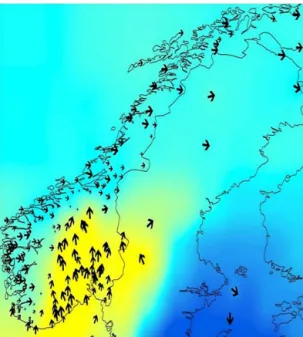
Atmospheric pressure data were obtained from the NCEP/NCAR reanalysis project (Kalnay et al., 1996) and include geopotential height data centred over Norway (0– 20◦E, 55–70◦N) for the 1000 hPa level (Z1000) and the 700 hPa level (Z700) at UTC at a spatial resolution of 2.5◦×2.5◦. Precipitation data for the period 1970–2008 for 175 stations distributed across Norway were extracted from the “European Climate Assessment & Dataset” (ECA&D, 2011) database. These stations and the time period were se-lected out of the 368 available stations for the region, such that no station had more than 50 days with missing data. The locations of the precipitation stations and the grid of geopo-tential heights are presented in Fig. 2.
Figure 2. Precipitation stations and grid of geopotential heights used to build the WT classifications for Norway.
method (Method 2) is inspired by Plaut et al. (2010) and be-gins by analysing the synoptic situations associated with in-tense precipitations at each station. This is accomplished by calculating the average synoptic situation for the 30 highest observed precipitations. The average active synoptic situa-tions can then be classified, which results in a grouping of the weather stations. Finally, for each group of precipitation sta-tions, an average synoptic situation corresponding to intense precipitation is computed based on all the synoptic situations of the class (30×ni, whereni is the number of stations in groupi). The third method (Boé and Terray, 2008), here
re-ferred to as Method 3, uses a direct classification of all days, using both the “ground fingerprint” and the synoptic situation as identified in the pressure field, following variance normali-sation. All three methods also included an additional weather type in the classification scheme to account for days without rain, so that all days within a continuous daily record could be assigned a weather type.
The three methods use the same variables for describ-ing the synoptic situation. As demonstrated in Brigode et al. (2013), it is useful to consider two levels for the pres-sure field description (the 1000 and 700 hPa geopotentials), and two points in time for these values (0 h on the day of interest and 0 h on the following day). These four variables have also been recommended by Obled et al. (2002) based on their evaluation of the performance of different combinations of these four fields for probabilistic precipitation estimation. All three methods have taken these four variables into use.
Two scores were used to assess the discriminating power of the classifications: the within-type variability and the Cramer score (Anderson, 1962). The Cramer score evaluates
Figure 3.Distribution of Cramer20 scores for the 76 COST733 classifications, as compared with the scores for the three classifi-cations described in Sect. 3.1.
the discriminating power of a WT classification in terms of the occurrence of rain vs. no rain, as applied in Bárdossy et al. (1995). To place the focus on performance with respect to heavy precipitation, as opposed to all values of precipita-tion, the Cramer coefficient can be estimated on days with a precipitation greater than a given threshold. In the work presented here a 20 mm threshold was used, and this “heavy rain Cramer” coefficient is referred to here as the “Cramer20 coefficient”. It is computed for each station and is then aver-aged on the whole domain to develop a score which can be used to compare the classification methods.
Figure 4.Dominant wind direction on the 30 days with the highest precipitation values at each station.
of the extreme precipitation events in western and northern Norway. In mid-Norway, the dominance of this wind direc-tion is limited and air coming from other direcdirec-tions can also induce extreme precipitation.
Three WT classifications produced by each of the three methods were used to develop preliminary rainfall proba-bilistic models for the SCHADEX applications for the At-nasjø and Krinsvatn catchments. These initial trials led to the choice of Method 1 for the weather type classification, although it performs slightly more poorly than Method 2 (Fig. 3). In addition, during this process it was recognised that some of the seven WTs could be combined into four weather patterns (WP), thus improving the robustness of the fitted distributions as more events were available for each WP. The assessment of this robustness could have been based on statistical scores (as detailed in Garavaglia et al. (2011)), but in this case the choice has been made using expert judg-ment. This simplification of the classification was found to have a negligible effect on the final SCHADEX estimates and was, thus, retained. The resulting four WPs used in the SCHADEX applications for Norway, including the eight un-derlying WTs on which they are based, are illustrated in Fig. 5.
3.2 Defining MEWP distributions for centred rainfall For the application of SCHADEX to a given catchment, two to four relevant seasons are defined within the year, and the seasonal record for the areal precipitation (constructed from local station-based precipitation data) is then split into sub-samples corresponding to each WP. An exponential law is fitted to the high quantiles of the central rainfalls
correspond-Figure 5.Three weather pattern groups representing seven weather types leading to extreme precipitation and one weather type (WT8/WP4) representing dry days.
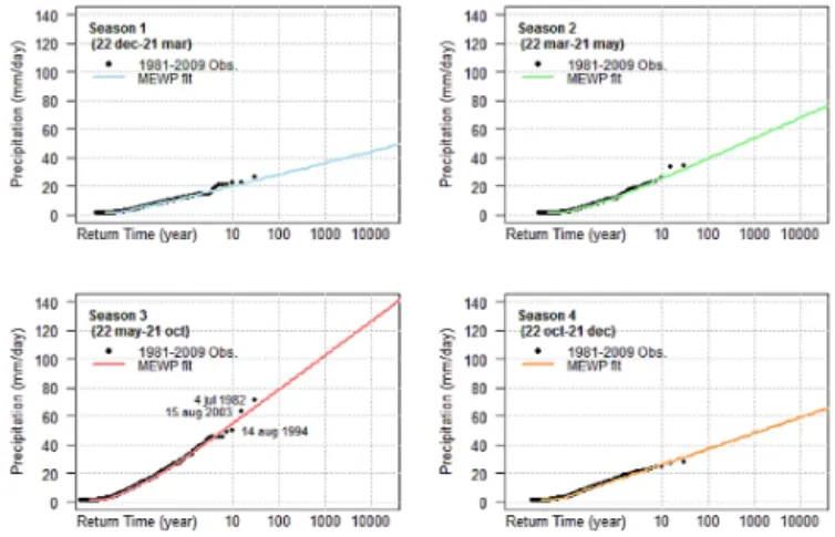
ing to each WP sub-sample (generally over the 70 % empir-ical quantile). For a given season, the MEWP distribution is composed of the marginal distribution associated with each WP, weighted by the relative frequency of occurrence of each WP for the considered season. In practise, alternative group-ings of months into seasons are often considered before the final set of seasonally fitted distributions is selected. Further details regarding the use of the MEWP for characterising ex-treme rainfall can be found in Garavaglia et al. (2010).
Figure 6.Example of WP-based fits for the June–October season at Atnasjø (right) with the resulting seasonal MEWP distribution (left).
with respect to the reliability and robustness of the extreme values analyses are presented in Garavaglia et al. (2011).
Ancillary probabilistic models complement the MEWP distribution to account for adjacent rainfall (i.e. the day be-fore and the day after the central rainfall) and for assess-ing the probability of the precipitation sequence which oc-curs during the few days preceding a centred event (i.e. the antecedent rainfall prior to the 3-day synthetic event). For the adjacent rainfall values (i.e. ratios relative to the central value), a contingency table is used to assign probabilities to the values drawn from the uniform distribution between 0 and 1. The boundaries between the classes used are chosen such that the classification is focused on the heaviest precip-itation events. The probability of the precipprecip-itation preceding the 3-day event is assessed based on the conditional probabil-ity of the simulated event, given the antecedent precipitation, specified as a stochastic variable described by the sum of two exponential distributions (Djerboua et al., 2004). The com-plete probabilistic scheme is described in detail in Paquet et al. (2013).
3.3 Hydrological modelling and analysis for the SCHADEX applications
For the SCHADEX applications, the MORDOR hydrologi-cal model, which is a lumped conceptual precipitation-runoff model also incorporating a sub-model for snow accumulation and melting processes (Garçon, 1996), was used. The MOR-DOR model was calibrated for the three Norwegian catch-ments based on a genetic algorithm with an objective func-tion designed to maximise both the Nash–Sutcliffe (N–S) ef-ficiency criterion and the fit between the observed and mod-elled empirical CDF of flow values. Calibration was based on a selection of 20 years between the period 1973–2010 for the three catchments, and the resulting N–S validation values were 0.85, 0.76 and 0.83 for Atnasjø, Engeren and Krinsvatn,
Figure 7.Seasonal MEWP distributions for Atnasjø.
respectively. Comparisons between simulated and observed daily inter-annual mean discharge are illustrated in Fig. 8 and indicate a good overall fit between modelled and sim-ulated values. The differences in the catchment flow regimes are also highlighted in this figure, as are the differences be-tween the general period of peak flows and the distribution of the annual maximum values by month. In particular, at Krinsvatn, there is a notable difference between the period of highest daily average values (i.e. April to May), which cor-responds to a period of seasonal snowmelt, and the monthly distribution of the annual maximum series, which indicates that high flows can occur throughout the year.
Figure 8.Daily inter-annual mean for both observed and modelled values and relative frequency of annual maxima by month.
3.4 SCHADEX stochastic simulations
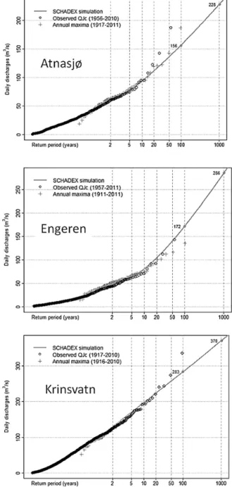
The SCHADEX simulations were run on a daily time step, corresponding to that of the calibrated hydrological model. For the three catchments, the simulation periods were ap-proximately 40 years in length, thus encompassing a wide range of hydrological situations, including the conditions producing the highest observed discharges. The simulation periods were also shorter than the entire period of the dis-charge record, as these were constrained by the availability of station-based precipitation data for creating an areal rainfall for use in defining the centred rainfall events and for running the hydrological model. The simulation periods were 1974– 2010, 1970–2008, and 1971–2010, for Atnasjø, Engeren and Krinsvatn, respectively. The stochastic simulations were run using the steps delineated in Paquet et al. (2013), and they produced∼2×10⁶flow events in each catchment. A com-parison of the distribution of these events with the annual maxima for the entire period of record and with the observed discharges associated with the centred rainfall events (QJc)
is illustrated in Fig. 9 for the three catchments. The results indicate good to very good correspondence between the sim-ulated SCHADEX distribution and the observed values. In some cases, the return periods corresponding to the highest observed events seem to be underestimated at Atnasjø and Krinsvatn. It must be kept in mind, however, that the empir-ical return period associated with the highest observed flows is very uncertain due to the length of the period of observa-tion. The SCHADEX distributions, as an alternative, indicate return periods of 270 and 407 years for the highest events at Atnasjø (1 June 1995) and Krinsvatn (31 January 2006), respectively. The SCHADEX estimation for Engeren gives a return period of 44 years for the historical flood of June 1995.
Figure 9.Distribution of daily discharge values based on SHADEX, as compared with the observed annual maxima and the observed discharges associated with centred rainfall events (QJc).
4 Methods applied for comparisons with SCHADEX results
parameter catchment model, PQRUT, driven by a predefined precipitation sequence. The sequence is constructed from es-timates of rainfall intensity for durations corresponding to the concentration time of the system of interest. These estimates are derived following the NERC (1975) method, as further developed for use in Norway (Førland, 1992). The method uses empirical growth curves to estimate intensity for vari-ous durations based on the so-called “M5” value (i.e. the 24 h rainfall with a 5-year return period), and in standard practice this estimate is based on a Gumbel extreme value distribu-tion. To simulate combined rainfall/snowmelt events, an ad-ditional contribution is added to the sequence, and this is de-rived from a simple temperature-based estimate of the max-imum melting rate for a given surface cover type. In more complex applications, a simple snowmelt model can be used to take account of differences in snow depth and depletion as a function of catchment elevation, but such applications are rare in practice. The combined precipitation/snowmelt sequence is then used as input to the PQRUT catchment re-sponse model.
The PQRUT catchment response model is usually run on an hourly time step, reflecting the small size and rapid re-sponse of the catchments often under consideration. Catch-ment response to the rainfall/snowmelt input sequence rep-resenting the extreme event is described using a three-parameter lumped “bucket”-type model in which outflow in response to inflow occurs either at a faster or a slower rate, depending on the value of accumulated depth relative to a threshold. As most extreme flood estimates for dam safety analyses in Norway are developed for ungauged catchments, values for the three PQRUT parameters are set based on three catchment physical characteristics (catchment steepness, ef-fective lake percentage, and normal runoff) using empirically derived formulas, although these can also be calibrated if sufficient precipitation and discharge data are available at the required temporal resolution. In most applications, the catchment is assumed to be fully saturated at the onset and throughout the simulated event, although an initial deficit volume can also be set. Further details regarding the method and its application can be found in Midttømme et al. (2011), and a summary of the method is also available in Wilson et al. (2011) in English.
moved forward by a day and a new simulation is run. This process is repeated through the entire observed series, such that the catchment response to the design precipitation un-der the range of soil moisture and snowmelt conditions is sampled. In Sweden, it is also assumed that the snow water equivalent at the commencement of the design precipitation has a 30-year return period. Further details of these meth-ods, which represent a type of long-term simulation, can be found in Bergström et al. (1992, 2008) and Veijalainen and Vehviläinen (2008). A significant advantage of this approach over event-based methods is that catchment response to the extreme precipitation sequence under a range of catchment conditions corresponding to differing saturation states and contributions from snowmelt is sampled during the simula-tion process.
4.3 Application of PQRUT and HBV-Design Flood to the study catchments
Figure 10. Application of GRADEX to Atnasjø, as described in Sect. 4.4.
to runoff in differing elevation zones within the catchment. In addition, following standard practice, the catchment was as-sumed to be fully saturated at the onset of the PQRUT sim-ulation. For the HBV-Design flood application, the Nordic version of HBV (Sælthun, 1996) was used, and HBV model parameters were estimated using the calibration procedures described in Lawrence et al. (2009). The HBV model vali-dations produced N–S efficiencies of 0.77, 0.77, and 0.78 for Atnasjø, Engeren and Krinsvatn, respectively. The HBV sim-ulations are run on a daily time step, and instantaneous peaks are estimated based on empirical formulas which take ac-count of flood season, catchment area and effective lake per-centage (Midttømme et al., 2011). Applying these formulae, the ratio of instantaneous peak to daily averaged discharge is 1.14, 1.07, and 1.37 for Atnasjø, Engeren and Krinsvatn, respectively. Note that the peak values based on these formu-lae give slightly higher values than those based on the actual analysis of sub-daily data (Sect. 3.3).
4.4 The GRADEX method and its application
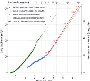
The GRADEX method has been used in France to esti-mate design floods for dam safety for more than 30 years. It is applied here as described in Duband and Garros-Berthet (1994), and the application is illustrated in Fig. 10 for At-nasjø. A sum of two exponentials (STE) distribution is first fitted to the daily precipitation of the season with the high-est flood risk of the catchment. Daily values are adjusted to account for the rain–snow limit, based on the daily mean air temperature values and the hypsometry of the catchment. The GRADEX parameter is the slope of the asymptotic exponen-tial law (the grey dotted line in Fig. 10) in a Gumbel plot
(here 8.4 mm/24 h). The discharge with a 10-year return pe-riod is then estimated based on the discharge annual max-ima (blue dots), available here from 1917 to 2010, using a Gumbel distribution. In this case, the 10-year discharge is 117 m3s−1. From this point, referred to as the pivot point, the daily discharge distribution is extrapolated up to a 10 000-year return period using the GRADEX parameter identified from the rainfall distribution (continuous grey line). The un-derlying hypothesis is that above this pivot point, which is assumed to correspond to highly saturated catchment condi-tions, the asymptotic growth of the daily runoff is the same as that for the daily rainfall (i.e. there is no additional storage available in the catchment), producing a parallel behaviour in the rainfall and the discharge distributions. To transform daily discharge into peak discharge, the daily discharge dis-tribution is multiplied by a peak-to-volume coefficient (here 1.04, shown as a red line).
5 Comparison of the SCHADEX results with other methods
5.1 Estimates for the 1000-year discharge
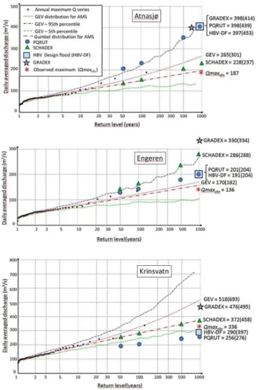
24 h precipitation (mm) 138 119 117 (97–151) 16 P1000=138
72 h precipitation (mm) 176 164 243 (202–282) 44 Snowmelt rate (mm d−1) 30 24 0 (0–9) Max=35 21
Catchment saturation 100 % 100 % 70 % (41–93 %) 100 % Date (or season) for Q1000 JJA 29/05/1988 Sep 01/06/1995
Krinsvatn
24 h precipitation (mm) 197 191 184 (162–213) 156 P1000=202
72 h precipitation (mm) 283 275 368 (304–448) 306 Snowmelt rate (mm d−1) 30 31 4 (0–24) Max=52 13
Catchment saturation 100 % 97 % 94 % (58–98 %) 98 % Date (or season) for Q1000 DJF 30/10/2005 Dec 31/01/2006
aValues for the SCHADEX method are given as the median value (modal value for date for Q1000), together with the 10th and
90th percentile values of the range of 104events producing a 1000-year discharge (Figs. 10, 11, and 12).bValues for snowmelt
and catchment saturation conditions for the maximum observedQare based on calibrated HBV simulations of the event.
Figure 11 indicates notable differences in estimates for the 1000-year discharge derived by the various methods. At Atnasjø, the “traditional” methods, PQRUT, HBV-DF and GRADEX, give much higher estimates than SCHADEX, which lies between the GEV and Gumbel estimates. At En-geren, all modelling methods give higher estimates than sta-tistical flood frequency analysis, particularly SCHADEX and GRADEX. In contrast, at Krinsvatn all of the modelling methods produce estimates which are lower than the GEV es-timate based on the annual maximum series. The SCHADEX estimates for Krinsvatn, however, correspond well with the fitted Gumbel distribution for all return periods considered. It should also be noted that PQRUT and HBV-DF, i.e. the methods based on an empirically estimated design precipi-tation sequence, lie below the 5 % confidence level for the GEV-based estimate for Krinsvatn.
5.2 Precipitation estimates
There is a range of factors related to both the precipitation input and the catchment conditions which contribute to the differences between the estimated 1000-year discharge mag-nitudes. A summary of these factors is given in Table 2 with reference to the PQRUT, HBV-Design Flood and SCHADEX methods, and they are also compared with the observed or
Figure 11.Comparison of estimates for the Q1000 discharges given by the various precipitation-runoff methods with statistical flood frequency analysis based on the annual maximum series.
than those used as input for PQRUT and HBV-Design Flood. At Engeren and Krinsvatn, even the 10th percentile of the distribution of the SCHADEX values is higher than the in-put precipitation values for PQRUT. It should also be noted that at Krinsvatn, the input 72 h precipitation for simulating the 1000-year event with PQRUT is less than that estimated as occurring during the period of the highest observed dis-charge.
5.3 Snowmelt and catchment saturation conditions Snowmelt rates for the PQRUT and HBV-Design Flood methods are very similar, particularly for Atnasjø and Krins-vatn, although these were derived differently. In the case of PQRUT, a value of 30 mm d−1 was assumed for all three catchments (see Sect. 4.3), whereas snowmelt is simulated by HBV using a temperature index method. In addition, changes in snow storage are simulated for each of 10 equal-area height zones, such that the value given in Table 2 is
Figure 12. Distributions of central (i.e. 1-day) and 3-day rain-fall volumes associated with the 104 simulated events producing a 1000-year discharge (Q1000). The values for the design precipi-tation sequence used in PQRUT are also indicated with solid dots.
Figure 13.Distributions of catchment saturation conditions and snowmelt rates associated with the 104simulated events producing a 1000-year discharge (Q1000) for the three catchments. The values simulated by HBV-DF for the event with the highest discharge are also indicated with “X”.
an average value for the entire catchment. The value given corresponds to the snowmelt rate during the highest sim-ulated discharge in response to the input precipitation se-quence. The maxima of all the simulated values are some-what higher, i.e. 27, 33 and 42 mm d−1for Atnasjø, Engeren and Krinsvatn, respectively. The median values of snowmelt for the SCHADEX simulations are significantly lower than those used in PQRUT and simulated by HBV. The full distri-bution of SCHADEX values for snowmelt associated with discharges with a 1000-year return period is illustrated in Fig. 13. These distributions for Atnasjø and Krinsvatn in-dicate that the highest 6–7 % of the simulated 1000-year discharges are associated with snowmelt rates similar to or higher than those of the PQRUT and HBV simulations. For Engeren, however, only very few simulations have rates sim-ilar to or higher than the 24 mm d−1simulated by HBV.
PQRUT assumptions and the HBV simulations, in that the saturation level is nearly 100 %. This is to be expected for a catchment in which peak flows occur primarily during the snowmelt season. For Krinsvatn, the median value is slightly lower, as is also the case for the HBV simulations. For En-geren, however, the median value for the catchment satura-tion is 70 %, indicating a significant potential for catchment losses at the onset of an event for many of the simulations.
5.4 Seasonality of 1000-year discharge
The SCHADEX simulations also highlight differences in seasonality with respect to vulnerability to extreme dis-charges between the catchments. The frequency distributions for the simulated Q1000 by month for the three catchments are shown in Fig. 14. At Atnasjø, the principal months asso-ciated with conditions producing 1000-year discharges are June, July and August. This agrees well with the season-ality of annual maximum flows (Fig. 8), the assumed sea-son for extreme events used for the PQRUT estimates (Ta-ble 2), the historical date for which the 1000-year precip-itation sequence produced the maximum discharge in the HBV-Design Flood simulations, and the date of the ob-served maximum discharge. The frequency distribution for the SCHADEX simulations at Krinsvatn indicates the au-tumn and winter months as the periods associated with most of the simulated 1000-year discharges, again in good corspondence with other simulations and observations and re-flecting the contrasting flood regime at this location. At En-geren, the SCHADEX simulations suggest July–September as the period most vulnerable to extreme flows, although a notable portion of such flows also occurs in May and June. The annual maximum series, on the other hand, are char-acterised by a dominance of peak flows in May under ob-served historical conditions. This is the case for both the en-tire period of record (1912–2011), and for the shorter period used for the SCHADEX simulations (1970–2008). The an-nual maxima indicate only one year out of 100 in which the annual maximum occurred outside of the period April– June, i.e. on 24 August 1912, and that value has a rank of 57 out of the annual maxima. Differences in the seasonal-ity of the SCHADEX 1000-year discharges relative to that
6 Discussion
components of flood processes through detailed models (pre-cipitation, snowmelt and precipitation-runoff) to infer the rel-evant conditions for extreme floods, which can differ from those represented by the highest observed discharges.
The periods used for the SCHADEX simulations, approx-imately 1972–2010 (full details in Sect. 3.4), are somewhat shorter than those used for statistical flood frequency analy-sis and the other modelling methods, 1957–2010 (Sect. 5.1), and this could in principle have an impact on the comparison illustrated in Fig. 11. Recent work (Brigode, 2013; Brigode et al., 2014) investigating the sensitivity of various components of the SCHADEX method to hydroclimatological variability indicates that as long as 20–30 years of good quality clima-tological data are used for developing the precipitation prob-abilistic model, the SCHADEX results tend to be relatively insensitive to the period considered for developing the rain-fall model (i.e. that presented in Figs. 6 and 7 for Atnasjø). This assumes, of course, a degree of stationarity over the en-tire period of interest, as well as a sufficient number of rain-fall events for the analysis. This latter factor was not an issue in the climatic regime considered here, but may become rele-vant for SCHADEX applications under semi-arid to arid con-ditions. The period used for hydrological model calibration, in contrast to that used for developing the precipitation prob-abilistic model, was found by Brigode et al. (2014) to have a relatively large impact on the final SCHADEX estimates.
The comparison of methods indicates several advan-tages of the SCHADEX approach over the more traditional precipitation-runoff methods for design flood analysis. Of primary interest to the practitioner is the capacity to generate a large range of possible rainfall magnitudes and catchment conditions that can produce an XX-year discharge, rather than requiring the assumption that an XX-year precipita-tion event produces the corresponding XX-year flood. This should lead to a better correspondence with results of statis-tical analyses of observed maximum flows, particularly for catchments with large contributions from snowmelt or which have variable levels of saturation at the onset of an extreme precipitation event. The SCHADEX methodology can also highlight potential seasonal flooding hazards not necessar-ily well represented by the observed annual maximum flow series. In addition, in contrast to continuous simulation meth-ods, the approach is not encumbered by the need to generate an excessively long time series using a weather generator, for example, in order to examine an ensemble of events with return periods of 1000 years and higher.
The further development of a SCHADEX-type methodol-ogy for use in regions dominated by extreme events caused by a combination of extreme rainfall and snowmelt requires a more in-depth scrutiny of factors contributing to differences in the snowmelt contributions simulated by the various meth-ods. Some of these differences may reflect differences in the hydrological model structure in that the Nordic version of HBV simulates changes in snow storage for 10 equal area height zones within the catchment, whereas the MORDOR
model has a lumped snow model for the entire catchment. Other differences, as discussed above, may reflect actual dif-ferences in the seasonality of potential extreme events rela-tive to the annual maximum series, although such a hypoth-esis can be difficult to verify. The seasonal behaviour, how-ever, could be evaluated further using a more in-depth peak over threshold analyses of observed discharge for this catch-ment.
For practical applications, a possible disadvantage of the SCHADEX approach relative to the other simulation meth-ods considered here is that it is a somewhat more complex tool and therefore may be more demanding of the user (see Paquet et al. (2013) for a description of the procedure). All three methods considered, i.e. PQRUT, HBV-Design Flood and SCHADEX, require areal estimates for the catchment rainfall as a daily time series. Given these data, the con-struction of the extreme precipitation sequence for PQRUT and for HBV-Design Flood applications is relatively simple for applications in Norway, relying on the equations given in Førland (1992) and requiring little prior experience. For SCHADEX, the rainfall probabilistic model is built for a given catchment and this entails fitting the MEWP model using a suitable distribution of seasons, setting up a contin-gency table for the ratios of the centred rainfall to the preced-ing and subsequent values, as well as buildpreced-ing a sub-model for antecedent rainfall. Although tools are available for these analyses within SCHADEX, the practitioner must have suf-ficient experience to be able to interpret the results and make required adjustments. Both HBV-Design Flood and SCHADEX require hydrological model calibration, and thus are more time-consuming than the simple three-parameter PQRUT model, which can be applied without calibration or calibrated based on observed hydrographs. In addition, both of the long-term simulation methods have longer computer run times, although these are nevertheless minimal as com-pared with continuous simulation methods.
The current version of SCHADEX requires observed daily discharge data for model calibration and hourly discharge data for assessing the peak-to-volume ratio for use in esti-mating instantaneous discharge values. Such data are rarely available in catchments for which design flood estimates are required. An advantage of the PQRUT model is that it can also be used in ungauged catchments. Further work to ex-tend the SCHADEX methodology to such catchments would represent a particularly significant advance in methods for design flood analysis.
15, 1087–109, 1995.
Bergström, S.: Development and application of a conceptual model for Scandinavian catchments, SMHI Report RH07, 1976. Bergström, S., Harlin, J., and Lindström, G.: Spillway design floods
in Sweden: I. New guidelines, Hydrol. Sci. J., 37, 505–519, 1992. Bergström, S., Hellström, S.-S., Lindström, G., and Wern, L.: Follow-Up of the Swedish Guidelines for Design Flood Determi-nation for Dams, Report No. 1, BE90, Svenska Kraftnät, 2008. Boé, J. and Terray, L.: A weather type approach to analysing winter
precipitation in France: twentieth century trends and influence of anthropogenic forcing, J. Climate, 21, 3118–3133, 2008. Boughton, W. and Droop, O.: Continuous simulation for design
flood estimation – a review, Environ. Modell. Software, 18, 309– 318, 2003.
Brigode, P.: Changement climatique et risque hydrologique: évalua-tion de la method SCHADEX en context non-staévalua-tionnaire. Doc-toral dissertation, Université Pierre et Marie Curie – Paris VI, 2013.
Brigode, P., Bernardara, P., Gailhard, J., Garavaglia, F., Ribstein, P., and Merz, R.: Optimization of the geopotential heights informa-tion used in a rainfall-based weather patterns classificainforma-tion over Austria, Int. J. Climatol., 33, 1563–1573, 2013.
Brigode, P., Bernardara, P., Paquet, E., Gailhard, J., Garavaglia, F., Merz, R., Mi´covi´c, Z., Lawrence, D., and Ribstein, P. Sensitivity analysis of SCHADEX extreme flood estimations to observed hydrometeorological variability, Water Resourc. Res., 50, 353– 370, 2014.
Cameron, D. S., Beven, K. J., Tawn, J., Blazkova, S., and Naden, P.: Flood frequency estimation by continuous simulation for a gauged upland catchment (with uncertainty), J. Hydrol., 219, 169–187, 1999.
Camici, S., Tarpanelli, A., Brocca, L., Melone, F., and Moramarco, T.: Design soil moisture estimation by comparing continuous and storm-based rainfall-runoff modeling, Water Resourc. Res., 47, WO5527, doi:10.1029/2010WR009298, 2011.
Djerboua, A., Duband, D., and Bois, P.: Estimation des lois des pré-cipitations extrêmes à partir de données journalières completes, La Houille Blanche, 3, 65–74, 2004.
Duband, D. and Garros-Berthet, H.: Design flood determination by the Gradex method, CIGB, ICOLD, 1994.
ECA&D: European Climate Assessment & Dataset, http://eca. knmi.nl/ (last access: November 2011), 2011.
Fleig, A.: Scientific Report of the Short Term Scientific Mis-sion – Anne Fleig visiting Électricité de France, Grenoble, 7–16 November 2011 (http://www.cost-floodfreq.eu/component/ k2/item/76-anne-fleig), 2011.
2011.
Garçon, R.: Prévision opérationnelle des apports de la Durance à Serre-Ponçon à l’aide du modèle MORDOR, Bilan de l’année 1994–1995, La Houille Blanche, 5, 71–76, 1996.
Grimaldi, S., Petroselli, A., Arcangeletti, E., and Nardi, F.: Flood mapping in ungauged basins using continuous hydrologic-hydraulic modeling, J. Hydrol., 487, 39–47, 2013.
Guillot, P. and Duband, D.: La méthode du gradex pour le calcul de la probabilité des crues à partir des pluies, Publication AIHS, 84, 560–569, 1967.
Kalnay, E., Kanamitsu, M., Kistler, R., Collins, W., Deaven, D., Gandin, L., Iredell, M., Saha, S., White, G., Woollen, J., Zhu, Y., Leetmaa, A., Reynolds, R., Chelliah, M., Ebisuzaki, W., Higgins, W., Janowiak, J., Mo, K. C., Ropelewski, C., Wang, J., Jenne, R., and Joseph, D.: The NCEP/NCAR 40-Year Reanalysis Project, Bull. Am. Meteorol. Soc., 77, 437–471, 1996.
Kuczera, G., Lambert, M., Heneker, T., Jennings, S., Frost, A., and Coombes, P.: Joint probability and design storms at the cross-roads, Australian J. Water Resour., 10, 63–79, 2006.
Lawrence, D., Haddeland, I., and Langsholt, E.: Calibration of HBV hydrological models using PEST parameter estimation, NVE Re-port no. 1-2009, 2009.
Midttømme, G. H., Pettersson, L. E., Holmqvist, E., Nøtsund, Ø., Hisdal, H., and Sivertsgård, R.: Retningslinjer for flombereg-ninger (Guidance for flood estimation), NVE Retningslinjer no. 4/2011, 2011.
NERC: Flood Studies Report, Volumes I-V, Natural Environment Research Council, London, 1975.
Obled, C., Bontron, G., and Garçon, R.: Quantitative precipitation forecasts: a statistical adaptation of model outputs though an ana-logues sorting approach, Atmos. Res., 63, 303–324, 2002. Paquet, E., Gailhard, J., and Garçon, R., Evolution of the GRADEX
method : improvement by atmospheric circulation classification and hydrological modelling, La Houille Blanche, 5, 80–90, 2006. Paquet, E., Garavaglia, F., Gailhard, J., and Garçon, R., The SCHADEX method: a semi-continuous rainfall-runoff simula-tion for extreme flood estimasimula-tion, J. Hydrol., 495, 23–37, 2013. Pathiraja, S., Westra, S., and Sharma, A.: Why continuous
simula-tion? The role of antecedent moisture in design flood estimation, Water Resour. Res., 48, W06534, doi:10.1029/2011WR010997, 2012.
Rahman, A., Weinmann, P. E., Hoang, T. M. T., and Laurenson, E. M.: Monte Carlo simulation of flood frequency curves from rainfall, J. Hydrol., 256, 196–210, 2002.
Sælthun, N. R.: The Nordic HBV Model, NVE Publication no. 07, 1996.
Tveito, O. E.: Climatological evaluation of circulation type classi-fications and precipitation in Norway/Fennoscandia, COST733 Final document, 2011.
Veijalainen, N. and Vehviläinen, B.: The effect of climate change on design floods of high hazard dams in Finland, Hydro. Res., 39, 465–477, 2008.