http://dx.doi.org/10.1590/0104-530X2196-15
Resumo: O presente trabalho apresenta um problema de dimensionamento e sequenciamento integrados para uma fábrica de grande porte de cimento para refratário. Foram abordadas três formulações matemáticas: duas presentes na literatura e uma proposta como alternativa às já existentes. Este estudo tem como objetivo comparar as formulações tanto em relação ao seu desempenho quanto à sua aplicabilidade como ferramenta de suporte à tomada de decisão. Uma dessas formulações utiliza variáveis contínuas e as outras são baseadas em variáveis indexadas no tempo. Estes modelos matemáticos abordam um conceito especíico de como as variáveis e parâmetros são deinidos, exigindo premissas e deinições particulares para se adequar ao problema real. A im de considerar os diferentes aspectos da situação prática, foram geradas várias instâncias a partir de distribuições uniformes, baseadas em informações reais. Extensivos testes computacionais foram executados e, com base nesses resultados, as modelagens foram avaliadas como ferramenta de apoio à decisão e as suas eiciências foram comparadas. Palavras-chave: Scheduling; Lot sizing; Planejamento e controle da produção; Modelos de programação matemática. Abstract: This work presents an integrated lot sizing and scheduling problem for a large refractory cement manufacturer. Three mathematical formulations were addressed: two already presented in the literature, and one proposed as an alternative to the existing ones. This study aims to compare these formulations with respect to their performance and applicability as a decision support tool. One of these formulations uses continuous variables, whereas the others are based on time-indexed variables. These mathematical models address the speciic concept of how variables and parameters are deined, requiring assumptions and particular settings to suit the real problem. In order to consider the different aspects of the practical situation, several instances were generated from uniform distributions based on real information. Extensive computational tests were run and, based on the results, the formulations were evaluated as a decision support tool and their eficiencies were compared.
Keywords: Scheduling; Lot sizing; Production planning and control; Mathematical programming formulations.
Integrated lot sizing and production scheduling
formulations: an application in a refractory
cement industry
Modelos integrados de dimensionamento e sequenciamento da produção: aplicação em uma fábrica de cimento para refratário
Fernanda de Freitas Alves1 Thiago Henrique Nogueira2 Rafaella de Souza Henriques2
Priscila Vieira de Castro2
1 Departamento de Engenharia de Produção, Universidade Federal de Minas Gerais – UFMG, Avenida Antônio Carlos, 6627, Pampulha,
CEP 31270-901, Belo Horizonte, MG, Brasil, e-mail: [email protected]
2 Departamento de Engenharia de Produção, Universidade Federal de Viçosa – UFV, Rodovia MG-230 – Km 7, CEP 38810-000,
Rio Paranaíba, MG, Brasil, e-mail: [email protected]; [email protected]; [email protected] Received Apr. 7, 2015 – Accepted Dec. 14, 2015
Financial support: FAPEMIG – irst author.
1 Introduction
Data from the Brazilian Ministry of Mines and Energy (Brasil, 2009) state that the refractory represents a segment of extreme importance, since
all industrial processes that use heat directly require
them, especially basic industries, as steel mills. According to the Magnesita Refratários (2015), the market of these products handles about US$ 25 billion per year all over the world, with the top six
companies representing nearly 40% of all global
refractories sales. It is predicted that consumption
of these products increases 3.3% until the year 2028. This work emerged from the need to seek
advantages in leverage of inancial results, considering
Integrated lot sizing and production scheduling formulations… 205
without interfering on the quality of the inal product.
The Operational Research comes as a tool to enable improvements in order to obtain a better organization of the production process, allowing a support to the decision making by mathematical modeling of real situations (Nogueira, 2008).
This study is the result of a real problem of lot sizing and production scheduling in a large refractory cement industry which is located in Contagem/MG. This company dedicates in mining, producing and marketing a wide line of refractory materials, being the third largest producer in the world and leader in
the Brazilian market of these products. It currently
employs about 6,400 employees and has production capacity of over 1.4 million of tones of refractories per year, achieving a sales revenue of 2.7 billion of reais in 2013, with selling to more than 1,000 customers in over 100 countries, resulting in an approximated
net proit of 30 million.
The objective of this study is to minimize the cost of inventory and unmet demand, usually caused by the lack of organization of the factory and its activities. The studied process is performed in continuous
low and it can be characterized as a single machine
problem which receives raw material and executes
the process, resulting in a inal product. In this
process, the bottleneck machine is responsible for the production rate and asymmetrical setup times between production lots are considered, i.e., they have time variations for each type of product/product family.
In this paper the problem is mathematically
formulated in three distinct ways, two which already
exists on the literature and a new one. In order to
compare the performance of the three formulations, the lower bounds, obtained by means of the LP (linear programming) relaxation, and the found optimum solution, when using commercial software, were discussed. Since the broached problem is NP-Hard,
with larger instances the computational time is a limit for the software in achieving the optimal solution. The LP relaxation was used for these formulations in order to meet the lower bounds, relaxing all their integer variables.
With the purpose of evaluating the proposed formulation, it was made a study comparing it with the other two approaches: a formulation with continuous variables based on Manne (1960), Santos (2006) and Carvalho & Santos (2006), and a reference formulation with time-indexed variables based on Toledo et al. (2007), Toso et al. (2009) and Ferreira et al. (2010). These formulations are applied to instances taken from real data and the results are compared.
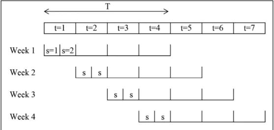
To achieve the objectives described herein it was used the rolling horizon approach, as shown in Figure 1. This technique consists in a differential to
reduce computational time, where the irst period is
divided into sub-periods and it will slide in time as planning is performed, with the scheduling detailed only for the immediate period. After, the horizon is rolled and the formulation is executed again, being updated with new information. The planning for future periods is done only for evaluation of the capacity. Thus, the number of variables in the formulation is drastically reduced (Carvalho & Santos, 2006).
Buxey (1989) highlights the uselessness in spending efforts with long periods, since that the uncertainty grows with the size of the auscultated time. The proposed planning formulation uses the planning horizon as discussed in Santos (2006).
This work is divided into six sections: section 1
gives an introduction to the broached subject. In section
2 it is done a literature discussion about this theme. The section 3 discusses the type of problem and the company’s particularities under study. The section 4 presents the proposed formulation and other ones
existing on the literature, comparing them. In section 5
the results of the presented formulations are discussed. Finally, the section 6 is about the conclusions of the study.
2 Literature review
Studies about production planning are found in large
quantity in the literature. According to Fernandes &
Santoro (2005) Production Planning and Control (PPC) problems are broached in three ways: considering only the production lot sizing, considering only the daily scheduling of items to be produced or considering these two aspects in an integrated way, i.e., the PPC integrated with scheduling. The latter form tries to join the long term planning to the short term one, making a weekly lot sizing of the items and daily scheduling of them.
The Table 1 shows in chronological order the main references in the literature used for this study. As it can be observed, about 10% of these works discuss the lot sizing problem. All of them have the objective of minimizing costs and one study uses for this the Lagrangian Relaxation.
Approximately 30% of the studies presented in the Table 1 are about the production scheduling problems. Considering the ones which present mathematical models, almost 70% of them use exact methods, such as Branch and Bound, and 30% heuristics. More than 40% of the scheduling problems aim to reduce the anticipation and delay costs, and the remaining 60% have various goals, such as minimizing the costs of the production resources and the production line setup.
Around 60% of the analyzed works discuss about the integrated PPC and scheduling problems. Considering the studies that have mathematical models, 40% of them use to solve the exact methods, such as Branch
and Bound and Branch and Cut, 50% use relax-and-ix
heuristic and the rest use Local Search algorithms and other heuristics. Concerning to the objectives of these studies, 45% of them minimize together the costs of inventory, unmet demand/backward and setup. The others have diverse objectives, including minimization of the extra hours and production costs. Around 80% of the works can be considered as a multi objective problem, and of these, 74% are integrated problems, 10% are lot sizing problems and 16% are scheduling problems.
It is possible to notice that, as the present study,
almost 90% of the works aim to minimize the costs, as the stock, unmet demand, production, delay or preparation costs. The problem under study is not found with the same focus on practical applications in the literature. Those with greater compatibility were found in the works of Toso & Morabito (2005) and
Henriques et al. (2010), which analyze scheduling
problems of discrete production lines, focusing on the
attendance of the inal products and determining the
lot sizing. Other studies that are similar in relation to
the objectives of this work are Araujo et al. (2007), Ferreira et al. (2009), Ferreira et al. (2010) and Stadtler & Sahling (2012).
The scheduling problems are widely studied in the
literature due to the dificulty level and applicability,
and they may extend to production scheduling, projects, vehicle routing, among others (Nogueira, 2014). The mathematical models of scheduling consist of allocating tasks and scarce resources to the products in order to meet the pre-established goal, setting
the sequence of goods production, as discussed in
Allahverdi et al. (2008), Pinedo (2012) and Leung (2004). Applications of these problems are also seen in Lawler (1976), Manne (1960), Du & Leung (1990), Sousa & Wolsey (1992), Tavares (2002), Santos & Massago (2007), Bustamante (2007), Yamashita & Morabito (2007), Chen & Askin (2009), Ramos & Oliveira (2011) and Rego (2013).
The lot sizing decisions are related to the amount
of end items. They should consider the inluence of
production factors, the costs related to the latters and
how these costs can inluence the PPC. The works
that address only the lot sizing problem can be seen in Brahimi et al. (2006) and Molina et al. (2013).
The studied problem is composed of an integrated lot sizing and scheduling formulation, as discussed in studies by Araujo et al. (2004), Carvalho & Santos (2006), Santos (2006), Toledo et al. (2007), Araujo et al. (2007), Toso et al. (2009), Ferreira et al. (2009), Ferreira et al. (2010), Bernardes et al. (2010),
Henriques et al. (2010), Stadtler (2010), Shim et al. (2011), Defalque et al. (2011), Clark et al. (2011),
Stadtler & Sahling (2012) and Seeanner & Meyr (2013).
The studies that use heuristics to address integrated formulations can be seen in Araujo et al. (2007) and Shim et al. (2011). The exact methods are also used to solve integrated problems, as it can be seen in Toledo et al. (2007). More detailed reviews on the exact methods can be seen in Nemhauser & Wolsey (1988), Pochet & Wolsey (2006), Arenales et al. (2007) and Wolsey (2008).
3 Problem
This study consists of an integrated lot sizing and scheduling problem with multi item, single machine, capacitated and the possibility of making stock and not meeting the demand. The database for the study was collected in a large refractory cement industry located in Contagem, Minas Gerais.
The details of the production process have greater emphasis on operational and organizational issues of the factory and by an analysis of them it is intended
to ind inconsistencies that might bring losses for the organization in terms of eficiency. This process has a linear low and it can be treated as a single machine
Integrated lot sizing and pr
oduction scheduling formulations…
207
Table 1. The used published works as well as its resolution method and objective.
Author Problem Solution Method Objective Function
Manne (1960) Scheduling - Minimize the makespan
Sousa & Wolsey (1992) Scheduling Cutting plane/Branch and Bound algorithm Minimize costs/Maximize proits
Tavares (2002) Scheduling -
-Araujo et al. (2004) Integrated Lot Sizing and Scheduling Local Search Algorithm Minimize inventory costs, backorder and setup costs
Leung (2004) Scheduling -
-Toso & Morabito (2005) Integrated Lot Sizing and Scheduling Relax-and-ix heuristic Minimize inventory costs and overtime costs Carvalho & Santos (2006) Integrated Lot Sizing and Scheduling Branch and Bound Minimize setup costs
Brahimi et al. (2006) Lot Sizing - Minimize production costs, setup costs, inventory holding costs and backlogging costs
Santos (2006) Integrated Lot Sizing and Scheduling Branch and Bound Minimize setup costs
Araujo et al. (2007) Integrated Lot Sizing and Scheduling Relax-and-ix heuristic/Local Search Algorithm
Minimize a penalty-weighted sum of product backlogs, inished inventories and setup changeovers
Bustamante (2007) Scheduling Branch and Bound Minimize the sum of earliness and tardiness costs Yamashita & Morabito
(2007) Scheduling Branch and Bound Minimize total cost allocation of project resources
Toledo et al. (2007) Integrated Lot Sizing and Scheduling Branch and Cut/Linear Relaxation Minimize production costs, setup costs and inventory holding costs Allahverdi et al. (2008) Scheduling - Minimize setup costs
Chen & Askin (2009) Scheduling Implicit enumeration algorithm Maximize proits
Ferreira et al. (2009) Integrated Lot Sizing and Scheduling Relax-and-ix heuristic Minimize the total sum of product inventory, demand backorder, machine changeover and tank changeover costs
Toso et al. (2009) Integrated Lot Sizing and Scheduling Relax-and-ix heuristic Minimize the costs of inventory, overtime and setup costs Bernardes et al. (2010) Integrated Lot Sizing and Scheduling Branch and Cut Minimize inventory costs, backorder and setup costs Stadtler (2010) Integrated Lot Sizing and Scheduling Branch and Bound Minimize inventory costs and setup costs
Henriques et al. (2010) Integrated Lot Sizing and Scheduling Branch and Bound Minimize inventory costs
Ferreira et al. (2010) Integrated Lot Sizing and Scheduling Relax-and-ix heuristic Minimize the total sum of the inventory, backorder and machine changeover costs Defalque et al. (2011) Integrated Lot Sizing and Scheduling Branch and Cut Minimize inventory costs, backorder and setup costs
Clark et al. (2011) Integrated Lot Sizing and Scheduling -
-Ramos & Oliveira (2011) Scheduling Hybrid evolutionary algorithm Minimize the sum of earliness and tardiness costs Shim et al. (2011) Integrated Lot Sizing and Scheduling Adapted heuristic Minimize the sum of setup and inventory holding costs
Stadtler & Sahling (2012) Integrated Lot Sizing and Scheduling Relax-and-ix/Relax-and-optimize heuristics Minimize inventory holding costs, setup costs and penalty costs for backorders
Pinedo (2012) Scheduling -
-Rego (2013) Scheduling Multi-objective algorithms Minimize makespan and total weighted lateness
Molina et al. (2013) Lot Sizing Modiied Lagrangian Relaxation Minimize inventory holding costs, backorder, setup costs and transportation costs
determining the process speed. It starts at the receiving
raw materials step and ends with the shipment of the
inal product to the customer.
The factory works in two turns of production and it has 32 silos available for input storage, of which 11 silos store raw materials that are common for many products and the other silos exchanged their types of raw materials according to the production
requirements. The receiving is done with bags that
are maintained in bins that are near to the production line entrance, which are supplied weekly (Figure 2 in section A).
The silos, Figure 2 in section B, are emptied after the production order and supplied with the necessary raw materials. The setup time for the product manufacturing is about 50 minutes, with 30 minutes for the silo unloading and 20 minutes for supplying it. There is preparation of one raw material at time, since there is a single device which transports the raw material to the silos. The bags with these materials are transported to the silos entrance and carried by an elevator to the empty silos, where the inputs are
ensiled. Each silo has 2,000 kg of capacity. After illing
these, the raw material is weighed by the hopper in the necessary amount for the receipt formation in the transport carriage, Figure 2 in section C. The silos are located over a trolley which receives the raw material after weighed and directs them to the mixer, Figure 2
in Section D, for subsequent bagging. The Figure 2 illustrates the production process of the studied
company, following the low: bin, ensilage, receipt
formation and mixer.
The ensilage has a great impact on idle time, since, as previously described, it spends about 50 minutes in each silo. The swap of product/product family
may result in changing raw materials in many silos, therefore, the greater the amount of silos that
requires change, greater the idle time. Furthermore,
product/product family which may cause contamination
increases the setup time, because of the requirement
for additional cleaning. Thus, the ensilage is crucial
for the scheduling due its inluence on idle time and available capacity. It is noteworthy that the discussed
data were strictly generated to consider the reality described here.
This study aims to create a greater integration between the tactical and operational decision making levels, seeking to facilitate the activities of PPC by means of the mathematical modeling. At the tactical level it is determined lot sizing and their respective
delivery date. At the operational level it is deined
the products/product family scheduling. According to Loveland et al. (2007), a formulation that communicates the tactical and operational decisions pursues to establish better communication and organization of
the shop loor.
Currently, the company’s PPC seeks to produce every week only the expected demand for this time interval, trying not to accumulate stocks of previous periods, but it incurs in the use of overtime when needed. The company believes that the demand uncertainties
are relatively large. However, PPC deines only the
need of production hours and it does not consider the time spent in scheduling. This scheduling is not planned in the initial program, leaving it to the operational level. Thus, many production plans set by
the PPC become infeasible on the shop loor or they require large amounts of overtime work. This is the
crucial problem to the company today. The proposed formulation should provide the anticipation of
Integrated lot sizing and production scheduling formulations… 209
production in periods when there is idle capacity,
and it seeks better production sequences, i.e., with fewer setups.
The company sales forecast is made by internal
and external forecasts. The irst week of planning has
real demands and by increasing the distance of the planning period, the demand is made by forecasts. All demands are available in the integrated management system of the company. An employee performs the
system to check the requests, returning information
about the inventory. At the end of this process, it is possible to determine how much manufacture of each product/product family.
The production scheduling is deined in the PPC
team meeting which, based on tacit knowledge,
deines the production sequence for the next few
weeks in order to reduce the idle time and ignoring the stock costs. This process spends around 8 hours per week, but it does not guarantee the optimality of the productions scheduling, i.e., it is not known how close the proposed solution is from the optimal
solution, since the proposed sequence only sets the
production scheduling, without considering the setup times. Then it is necessary to make additional calculations to check the feasibility of the demand meeting and delivery dates obedience.
It is interesting to highlight that there is no interaction
between the tactical and operational decision levels in determining the amount of goods to be produced. Therefore, there is no guarantee that the production
set by the PPC can be sequenced and manufactured. The sales orders are supplied by the inished product
inventories or, if there are not the good in stock, they
are converted into production orders. The sequencing
of these production orders should be done respecting the established demand.
The company has a 5% rate of overdue delivery because of the lack of capacity on the production line. Currently, 20% of the available line time is used in the machine setup, thus, minimizing this time results in increasing the capacity and reducing the delays in delivery. Therefore, there is a need to create a mathematical model that organizes the production line, reducing the preparation time and increasing the time for production. This formulation should look for
the best production sequence in order to minimize
the costs inherent to the process.
The PPC has chosen to work with a planning period of only seven days, even providing four weeks to the sales department. This period was chosen based on the information reliability, and in the current week
the requests are made based on actual demands.
The PPC department, to increase productivity, allows anticipating the production and attending the orders before the expected date, however, this can lead to unnecessary stock.
4 Proposed formulations and
solution method
This study presents three mathematical models for integrated lot sizing and scheduling with the objective of minimizing the unmet demand and inventory
costs, considering sequence-dependent setup times.
These models are: one with continuous variables, one reference approach with time-indexed variables and a new formulation proposed by the authors.
The irst approach, denominated Mixed-Binary-Integer
Linear Programming with Continuous Time Horizon
(MBILP-CH), is based on Manne (1960), Carvalho
& Santos (2006) and Santos (2006). This formulation presents continuous, integer and binary variables and a continuous time planning horizon. The second approach is based on works of Toledo et al. (2007), Toso et al. (2009) and Ferreira et al. (2010). This is denominated
Mixed-Binary-Integer Linear Programming with Discretized Time Horizon (MBILP-DH) and it presents
time-indexed variables, with the planning horizon discretized into s sub-periods. In this formulation, the s parameter is at most equal to the number of product families j, thus all families can be produced
(but do not need to be). Finally, the formulation
proposed, denominated Mixed-Binary-Integer
Linear Programming with Discretized Time Horizon
(MBILP-DHP), inspired by previous formulations
presented and by the works of Sousa & Wolsey (1992)
and Henriques et al. (2010).
The MBILP-DH and MBILP-DHP formulations
present time-indexed variables (discretized planning horizon), and as analyzed by Keha et al. (2009)
this implies in tighter bounds. In the MBILP-DHP
formulation the time is discretized in s sub-periods
with size equal to the production capacity in hours
available. This increased planning horizon leads to a larger number of variables and constraints than
MBILP-DH, and consequently, it restricts the size
of instances that can be solved.
Keha et al. (2009) and Unlu & Mason (2010) showed that the lower bounds obtained from the formulations based on the proposal of the Sousa & Wolsey (1992) were strong, but the LP relaxations are harder to solve compared to the other formulations. However, the computational experiments from De Paula et al.
(2010) suggest that when sequence-dependent setup
times are introduced, the LP relaxation bounds in the time-indexed formulation are not as strong. Nogueira (2014) highlights this fact and proposes a family of
valid inequalities to improve the lower bounds obtained with sequence-dependent setup times. Furthermore,
4.1 Problem modeling
The MBILP-CH and MBILP-DH formulation are
based on Manne (1960), Carvalho & Santos (2006), Santos (2006), Toledo et al. (2007), Toso et al.
(2009) and Ferreira et al. (2010). The MBILP-DHP
formulation is a new proposal, inspired by the works
of Sousa & Wolsey (1992) and Henriques et al. (2010).
All formulations consider the following considerations:
i) the studied problem is treated as a single machine problem, considering rolling horizon strategy; ii) the
lots have different sizes and its sequence impact on
the total time spent on setups. When there is no risk of contamination between families the setup time is short, otherwise it is longer and compromises the total time available for production. The sets for the formulations are:
- J refers to the set of product families to be produced, with J= …{1, ,j}.
- T refers to the set of periods in the planning horizon, with T= …{1, ,t}.
- S refers to the set of sub-periods in the planning horizon, with S= …{1, ,s}.
The indexes used in the mathematical models are:
- i refers to the product family considered, such that i∈J.
- t indicates the period of the planning horizon considered, such that t∈T.
- s indicates the sub-period of the planning horizon considered, such that s∈S.
The parameters considered for the formulations are:
- dit: Demand of the product family i in period t.
- Smi: Minimal setup time to produce the product family i.
- pi: Processing time of the product family i.
- Ct: Total capacity in hours in period t.
- Stij: Setup time to changeover from the product family i to the product family j.
- Hi: Inventory cost of the product family i.
- Bi: Backorder cost of the product family i.
- M: Large value, which is given by the total time taken to produce all the demand of the
irst week of planning plus the maximum time
spent for preparing the production of the product family i to the product family j, as can be seen in Nogueira (2014), which is given by:
1
( i i) j J ij.
i J i J
M p d max∈ St
∈ ∈
=
∑
+∑
(1)The decision variables used in the formulations are:
- Iit: Continuous variable that indicates the amount in stock of the product family i in period t.
- qit: Continuous variable that indicates the amount produced of the product family i in period t.
- Iit−: Continuous variable that indicates the
backorder of the product family i in period t.
- ri: Continuous variable that indicates the starting time of the production of the product family i.
- b
ijs: Binary variable that indicates the production (bijs = 1) or not (bijs = 0) of the product family j
after the production of the product family i in sub-period s.
- vit: Binary variable that indicates the production (vih = 1) or not (vih = 0) of the product family i
in period t.
- xis: Binary variable that indicates the production (xis = 1) or not (xis = 0) of the product family i
in sub-period s.
- yij: Binary variable that indicates the production (yij = 1) or not (yij = 0) of the product family j
after the production of the product family i.
4.1.1 MBILP-CH – mixed-binary-integer linear programming with continuous time horizon
The formulation is evidenced below:
(
)
,
i it i it i J t T
Minimize H I B I−
∈ ∈
∑
+ (2)Subject to:
, 1 , ,
it i t it it it
I =I − + − + ∀ ∈ ∀ ∈q d I− i J t T (3)
(it i it i) t 2 , i J
v Sm q p C t t
∈ + ≤ ∀ = …
∑
(4), 2 , it i t it
q p ≤C v ∀ ∈ ∀ = …i J t t (5)
(
)
1 1 1 , , ,
j i ij i i i ij
r ≥ +r St v +p q −M −y ∀ ∈ ∀ ∈i J j J i≠j (6)
1 , , ,
ij ji
y +y = ∀ ∈ ∀ ∈i J j J i≠j (7)
1 1 1 ,
i i i i
r+p q ≤C v ∀ ∈i J (8)
{ }0,1 , , , ij
y ∈ ∀ ∈ ∀ ∈i J j J i≠j (9)
{ }0,1 , , it
v ∈ ∀ ∈ ∀ ∈i J t T (10)
, , 0 , ,
it it it
q I−I ≥ ∀ ∈ ∀ ∈i J t T (11)
0 . i
Integrated lot sizing and production scheduling formulations… 211
The problem aims to minimize the inventory costs and the backorder costs, as shown in the Constraint
2. In the Expression 3 we have the line balancing
constraint in which the amount of stock Iit of the product family i in the end of period t is equal to
the stock of the previous period Ii,t–1 increased of the production of period t, qit, and backorder of the same period Iit−, reducing the demanded quantity dit. The Constraint 4 limits the capacity of the factory, showing that the minimum amount of hours of setup
(it i) i J
v Sm ∈
∑
plus the total production time ( it i) i Jq p ∈
∑
ofthe product family i must be smaller than the total time capacity of the factory Ct, from the period 2.
If the product family i is produced in the period t, the total time qit pi for its production must be less than the total capacity of the factory Ct vit, as shown in the Constraint 5, being valid from the second planning
period. The Constraint 6 requires that the production
start date rj of the product family j is equivalent to
the starting date ri of the production of the product family i plus the time spent in preparation for the exchange of the product family i to the j,Stij vi1 added to the total amount of production time of the product family i in the irst time period, pi qi1. Note that rj
must obey to this expression when the manufacture of the product family j occurs after the manufacture of the product family i (yij = 1). Otherwise, (yij = 0), the Expression 6 will have the subtraction of a very large value, denoted by M, so that it will not restrict the amount rj. The Constraint 7 states that, within a certain range of time, there will be exchange from the product family i to j or the contrary, i.e., it will
be only one exchange during this period. In the
Constraint 8 it is possible to see that the production beginning time of i plus the lead time of this product family should be less than the period 1 capacity, if the product family i is produced in this period.
The Constraints 9, 10, 11 and 12 deine the domains
of the variables.
4.1.2 MBILP-DH – mixed-binary-integer linear programming with discretized time horizon
Following the modeling for this formulation.
,
( i it i it) i J t T
Minimize H I B I−
∈ ∈
∑
+ (13)Subject to:
, 1 , ,
it i t it it it
I =I − + − + ∀ ∈ ∀ ∈q d I− i J t T (14)
(it i it i) t 2 , i J
v Sm q p C t t
∈ + ≤ ∀ = …
∑
(15)( 1 ) 1 , , ,
( ijs ij) i i , i J j J s S i j i J
St q p C
b
∈ ∈ ∈ ≠
∑
+∑
∈ ≤ (16), 2 ,
it i t it
q p ≤C v ∀ ∈ ∀ = …i J t t (17)
1 1 ,
i i is
s S
q p C x i J
∈
≤
∑
∀ ∈ (18)1 , is
i J
x s S
∈ = ∀ ∈
∑
(19), 1 1 , , 2 , ,
ijs xi s xjs i J j J s s i j
b ≥ − + − ∀ ∈ ∀ ∈ ∀ = … ≠ (20)
{ }0,1 , , , ,
ijs i J j J s S i j
b ∈ ∀ ∈ ∀ ∈ ∀ ∈ ≠ (21)
{ }0,1 it
v ∈ ∀ ∈i J, ,∀ ∈t T (22)
{ }0,1 , , is
x ∈ ∀ ∈ ∀ ∈i J s S (23)
, , 0 , .
it it it
q I−I ≥ ∀ ∈ ∀ ∈i J t T (24)
The objective function shown in the Constraint 13 is the same as already discussed in the Constraint 2, as well as the Constraints 14 and 15, which have the same meaning of Constraints 3 and 4, respectively. Given the production in sub-periods,
the preparation of the production line is required
when the production of a product family j in the sub-period s begins after the end of the production of the family i, considering a total capacity into
productive time in the irst planning period, C1, the sum of the setup times and production times, as shown in the Expression 16. The Constraint 17 shows that the time for the production of each product family
i in a given period of time should be less than the total capacity in time Ct in period t. In the Constraint
18 we have that if the product family i is produced in period 1 its production time should be less than the capacity in this time period. The Constraint 19 shows that only a product family shall be produced by sub-period s. The Constraint 20 shows that there will be only production of the product family j after the production of the product family i in the sub-period
s if there are production of i in sub-period s-1 and production of j in sub-period s, i.e., there will be a change in the product family i to the product family
j. The Expressions 21, 22, 23 and 24 deine the
domains of the variables.
4.1.3 MBILP-DHP – mixed-binary-integer linear programming with discretized time horizon
The proposed formulation, as already mentioned, is
based on Sousa & Wolsey (1992) and Henriques et al.
(2010). This is a new formulation, inspired by
scheduling problems, however, requiring particular settings and deinitions. For this formulation a new
- ai: Product family i production rate in each sub-period.
Are also used the new variables:
- zis: Binary variable indicating the beginning (zis = 1) or not (zis = 0) of the product family i
production in sub-period s.
- wis: Binary variable indicating the end (wis = 1) or not (wis = 0) of the product family i production in sub-period s.
The proposed formulation is presented below.
,
( i it i it) i J t T
Minimize H I B I−
∈ ∈
∑
+ (25)Subject to:
, 1 , ,
i t it it it it
I − + + =q I− d + ∀ ∈ ∀ ∈I i J t T (26)
( it i it i) t 2 , i J
v Sm q p C t t
∈ + ≤ ∀ = …
∑
(27), 2 ,
it i t it
q p ≤C v ∀ ∈ ∀ = …i J t t (28)
1 ,
i i is is is
s S s S s S
q a sw sz z i J
∈ ∈ ∈
= − + ∀ ∈
∑
∑
∑
(29),
is is
s S s S
w z i J
∈ = ∈ ∀ ∈
∑
∑
(30)1 , is
s S
z i J
∈ ≤ ∀ ∈
∑
(31)( )
min 1,
, 1 , , , ,
ij i
s St p s
is j ss
ss s
w z s S i J j J i j
+ + −
=
+
∑
≤ ∀ ∈ ∀ ∈ ∀ ∈ ≠ (32)2
, 1 , 2 1
1 , , 1 , 2 , 2 1, ,
s
is i s j s
s s
w z z i J j J s S s S s s i j
= ≥ + − ∀ ∈ ∀ ∈ ∀ ∈ ∀ ∈ ≥ ≠
∑ (33)
2
, 1 , 2 1
1 , , 1 , 2 , 2 1, ,
s
is j s i s
s s
z w w i J j J s S s S s s i j
= ≥ + − ∀ ∈ ∀ ∈ ∀ ∈ ∀ ∈ ≥ ≠
∑ (34)
{ }
, 0,1 , ,
is is
w z ∈ ∀ ∈ ∀ ∈i J s S (35)
{ }0,1 , , it
v ∈ ∀ ∈ ∀ ∈i J t T (36)
, , 0 , .
it it it
q I−I ≥ ∀ ∈ ∀ ∈i J t T (37)
The Constraints 25, 26, 27 and 28 have the same meaning as the Constraints 2, 3, 4 and 5, respectively. The amount to be made of the product family i in
the irst period is given by the Constraint 29, in which this quantity is calculated based on the time
spent and in the production rate, ai. The Constraint 30 ensures that the entire product family i which has its production started must be completed, guaranteeing the processing end of all items started. The Constraint 31 determines that each product family has its production started only once in all
sub-periods s. The Constraint 32 ensures that if the product family i is allocated to a sub-period s, so no other product family j can be allocated until the end of this sub-period, while respecting the total capacity
of the irst week of planning. In the Constraint 33 it
is set that between two beginnings of production will always be an end and the Constraint 34 determines that between two endings of production will always be a start. The Constraints 35, 36 and 37 present the domains of the variables.
The proposed formulation, MBILP-DHP, presents
homogeneity in its time of the sub-periods, since the length thereof does not depend on the lead time of each product family. Thus, directly by the values of variables zis and wis it is possible to determine the chronological position of certain product family, as well as the precedence relations of the whole production.
Both the MBILP-CH and the MBILP-DH only show
the start date of the production of each product family, there being no temporal detail during manufacturing. This fact imposes that the production of all demand for certain product family occurs once in the period.
In addition, attention should be given to the fact that the MBILP-CH presents the parameter M, a large number, which is often determined arbitrarily, worsening the limits obtained.
Like the irst two formulations presented, the latter
limits by the Restriction 31 that, in all sub-periods, a product family initiate its production only once. This
assumption was adopted so that the MBILP-DHP
possesses the same characteristics of other formulations discussed here. However, if it has been suppressed, the formulation is able to realize interruption in the production of a product family to begin another and,
where possible, complete the production of this irst,
characterizing the preemptive scheduling.
Analyzing the problems of PPC, this characteristic
can beneit managers to adapt the production more
easily to unexpected and urgent demands of some products. Thus, the production of these can be prioritized without compromising the remaining scheduling. The imposition that the entire necessary amount of a product/product family should be manufactured at a single time per period may generate some practical complications.
5 Computational results
Extensive computational experiments are performed to identify the strength and the weaknesses of each proposed formulation as a support decision tool.
In order to analyze the performance of the mathematical formulations same parameters will be varied. A speciic
Integrated lot sizing and production scheduling formulations… 213
5.1 Benchmarking
Three different classes of instances are created based on real data. All instances classes have four
weeks for the planning horizon. In the MBILP-DHP
formulation, each week is divided into 112 sub-periods of 1 hour (2 shifts of 8 hour for each day of the week).
In MBILP-DH formulation each week is divided in an amount equal to the number of product families
to be produced. Therefore, in this formulation, the
size of each sub-period is lexible, i.e., it will always depend on the number of product families that will be produced in each week. For all formulations were considered the following distinct product family
quantities: 2, 3, 4, 5, 6, 7, 10, 15 and 20. Furthermore,
the inventory of any product family at the start of the planning horizon is zero.
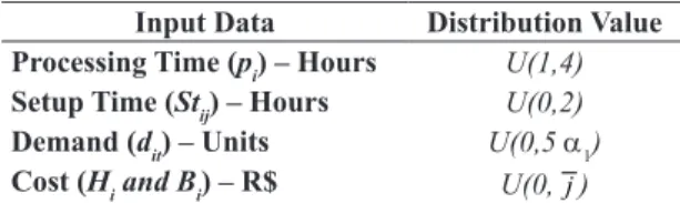
All parameters of the instances are randomly generated from a uniform distribution and their
minimal and maximal values are based on speciic
scale parameters listed in Table 2.
The j parameter refers to the total number of
product families in J. The values of the demand for each family, the processing time, the setup times, the cost of inventory and the cost of backorder are based on real data. The demand for each family is generated by three different ways (Classes 1, 2 and 3) to capture
several aspects of real situations and their inluences.
The amount is generated by a parameter a1 with values 0.75, 1.50 and 3.00 for each class respectively. For each class, three independent instances are considered with size j∈{2, 3, 4, 5, 6, 7,10,15, 20 .} Thus, 81 instances are randomly and independently generated. All instances
are slightly modiied to satisfy the triangle inequality
(Stij≤Stil+ ∀ ∈ ∀ ∈ ∀ ∈Stlj i J, j J, l J i, ≠ ≠j l). The M value
was deined by Equation 1.
5.2 Results
The mathematical formulations were modeled and solved using AMPL and CPLEX 12.1 with default settings. The experiments were run on a Windows 7 with a single 2.2 GHz processor and 4GB memory. The runs were concluded after one hour of CPU time.
5.2.1 Speciic results
5.2.1.1 Validation of the formulations solutions
In order to evaluate and to compare the solution of
the three formulations, this section aims to analyze the solutions of each one, taking as input the same
data. First it was chosen one instance problem with three product families to be processed, with four sub-periods. All formulations managed to solve at
optimality and the resolution times for MBILP-CH, MBILP-DH and MBILP-DHP were, respectively,
0.05, 0.55 and 68.25 seconds.
The lot sizing variables obtain identical results for the three formulations, satisfying the demand without any inventory or backorder. However, these formulations present different solutions for the
scheduling of the irst period for the same instance
problem, emphasizing the difference between them.
For the MBILP-CH the product families schedule
is 2-3-1, with their start times (ri) 0, 30 and 38. In this
formulation it is possible to identify directly by decision variables the schedule and the start times. Although there is no complexity in these calculations, it is clear
that this formulation requires auxiliary procedures to
identify the production completion times.
The MBILP-DH presents the optimal schedule
3-1-2. The solution shows the number of sub-periods
equals to the amount of product families, therefore
there is no temporal notion about the production beginning and end of each product family. Again,
this formulation also requires auxiliary procedures
to provide more details of the solution.
For the MBILP-DHP the product families schedule
is 2-1-3, with their start times (zis) and completion times (wis): 3 and 30, 45 and 96, 106 and 111, respectively. The decision variables allow a temporal notion of the schedule, and it is evident by them that the solution presents slack, therefore, if necessary, more product
families can be added for the irst period.
The formulation MBILP-DHP has longer resolution
time than the other formulations, however the elimination of the Restriction 31, as already mentioned, enables
the preemptive scheduling. This provides lexibility to
start and complete the production of a product family more than once in the same period. This choice can
be useful to anticipate the production of subsequent
periods, if the cost of backorder is higher than the cost of the generated inventory.
5.2.1.2 Comparation with company’s results
As mentioned, the company decides the schedule
of the families to be produced just for the irst week of
the planning horizon, not anticipating the production of next weeks, preferring to incur in overtime when necessary. This practical may cause idleness in production line and backorders.
This study aims to deine mathematical formulations
that allow the studied company anticipates the production of other weeks for the previous weeks with idleness, reducing the costs of the backorder and delivery delays. Furthermore, the forecasts for more Table 2. Distribution values of the instances.
distant periods are likely to change once the horizon is rolled forward and managers often have to revise the plans to cope with disruptive events. For this, the production planning should be done considering a rolling horizon, scheduling the product families for
the irst week and just deining the lot sizing for the
remaining weeks.
In general, the mathematical formulations present
an average delay of 0% for the product families to instances of the classes 1 and 2 and 7% for the Class 3, the last has tighter demand in relation to other classes. The total average delay presented by formulations is approximately 2%, while the company historical
average delay is 4%. It is noteworthy that the data
is based on real historical values of the company, but there is no guarantee that the behavior exhibited by the mathematical formulations is exactly the identical as the real company results, even if the instance problems used in this study were based on real historical data.
5.2.2 General results – performance evaluation of the formulations
To analyze the differences between the formulations, it was compared the optimality GAP (GAPInteger) within 3,600 seconds, the LP relaxation GAP, CPU times and its dimensions. The LP relaxation gap (GAPRelax)
is deined as the relative difference between the best
integer solution found for each instance and the LP relaxation value, divided by the best integer solution. The results of the experiments and analysis are presented in Tables 3 and 4. The Table 3 depicts the average GAP results and the average computational times for the presented formulations considering each instance class problem, while Table 4 shows the dimension of the formulations.
In Table 3, the irst two columns refer to the instance class and the number of product families. For each instance class its average and its standard deviation are calculated. The TRelax and TInteger indicate the average CPU times for the LP relaxation and
the mixed-integer programming (MIP) problem,
respectively. The “% Inst. Resol.” is the percentual of the instances solved within 3,600 seconds for LP
relaxation and MIP problem.
As an example, the “Class 1” and the “Product Family 20” in Table 3 indicate that 20 distinct product families are considered, with its characteristics
deined in the “Class 1” in “Section 5.1”. Therefore,
as already presented, three results were generated for the “Class 1” and the “Product Family 20” and its averages for the GAPs and the computational times are calculated. Furthermore, its average and standard deviation values are calculated for each instance class to compare the performance of the formulations.
For instance classes 1 and 2 with up to 5 product families all analyzed formulations have GAP near to 0%, whereas them managed to optimality solve in
most cases, for both LP relaxation and MIP problem. It is also observed a reduced computational time, which justiies the use of the formulations for a small number of product families. In the Class 3, the LP
relaxation of the mathematical formulations presents higher GAP values than classes 1 and 2. The higher
Relax
GAP is presented by MBILP-CH with value of
75.6%, however this formulation has computational time near to 0 seconds for all instances. The results of the Class 3 were expected due to have a tighter demand than other classes.
For the instance classes greater than 5 product
families, the MIP formulation MBILP-DH has GAP
near to 0% for all problems. On the other hand, for
large problem instances the MBILP-CH presents worse lower bounds than MBILP-DH. The MBILP-CH has
GAP values near to 100% with similar computational
time to MBILP-DH. The LP relaxation also presents similar GAPs to MIP problems, having few instances
with solutions near to the optimal.
The formulations MBILP-CH, MBILP-DH and MBILP-DHP solve 100%, 100% and 67%
of the instance problems for the LP relaxations,
respectively, and 72%, 77% and 41% for the MIP
formulations. As the size of the input data increases, the GAP and the computational time increase faster
for MBILP-DHP, solving smaller number of LP and MIP instances than other formulations. This is due to
number of constraints and variables associated with
MBILP-DHP which increase the model’s size faster than other formulations. It must be highlighted that in
several occasions the formulation was unable to load
the whole problem into the solver. In those cases the GAP and its computational time were deined by “-”.
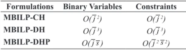
The Table 4 presents the order of complexity for each formulation. For the formulations, “Binary Variables” indicate the number of associated variables and “Constraints” the number of associated constraints.
The formulation MBILP-DH presents in its worst
case, s=j, therefore, its representation is only in function of j in Table 4. The complexity of the
formulations MBILP-CH and MBILP-DH in this
article have a polynomial number of constraints and variables in the input data. However, this is not the case
for MBILP-DHP, as they also are strongly dependent
on j and s. It is worth noting that as sj, s∝j (see
Keha et al. (2009) for more details), MBILP-DHP
formulation will increase its size faster than other
formulations. In this paper the size of the s was
deined in “Section 5.1”.
As it can be seen in Table 4, the MBILP-CH has a smaller number of constraints and variables than
other presented formulations. The MBILP-DH has
Integrated lot sizing and pr
oduction scheduling formulations…
215
Table 3. Results related to each class and each product family for formulations MBILP-CH, MBILP-DH and MBILP-DHP.
Class Product Family
MBILP-CH MBILP-DH MBILP-DHP
GAPRelax TRelax % Ins.
Resol GAPInteger TInteger
% Ins.
Resol GAPRelax TRelax
% Ins.
Resol GAPInteger TInteger
% Ins.
Resol GAPRelax TRelax
% Ins.
Resol GAPInteger TInteger
% Ins. Resol
1 2 0.0% 0.0 100.0% 0.0% 0.1 100.0% 0.0% 0.1 100.0% 0.0% 0.1 100.0% 0.0% 0.8 100.0% 0.0% 7.5 100.0% 1 3 0.0% 0.0 100.0% 0.0% 0.1 100.0% 0.0% 0.1 100.0% 0.0% 0.1 100.0% 0.0% 2.4 100.0% 0.0% 51.6 100.0% 1 4 0.0% 0.1 100.0% 0.0% 0.1 100.0% 0.0% 0.1 100.0% 0.0% 0.1 100.0% 0.0% 5.2 100.0% 0.0% 109.2 100.0% 1 5 0.0% 0.0 100.0% 0.0% 0.1 100.0% 0.0% 0.1 100.0% 0.0% 0.1 100.0% 0.0% 9.0 100.0% 0.0% 315.4 100.0% 1 6 0.0% 0.0 100.0% 0.0% 0.1 100.0% 0.0% 0.1 100.0% 0.0% 0.1 100.0% 0.0% 15.2 100.0% - - 0.0% 1 7 0.0% 0.1 100.0% 0.0% 0.1 100.0% 0.0% 0.1 100.0% 0.0% 0.1 100.0% 0.0% 20.9 100.0% - - 0.0% 1 10 0.0% 0.1 100.0% 0.0% 0.1 100.0% 0.0% 0.1 100.0% 0.0% 0.1 100.0% - - 0.0% - - 0.0% 1 15 99.9% 0.1 100.0% 100.0% 3600.0 0.0% 84.8% 0.1 100.0% 40.0% 1212.9 67.0% - - 0.0% - - 0.0% 1 20 99.9% 0.1 100.0% 100.0% 3600.0 0.0% 57.6% 0.2 100.0% 26.0% 3600.0 0.0% - - 0.0% - - 0.0%
Average 99.9% 0.0 100.0% 22.2% 800.1 78.0% 15.8% 0.1 100.0% 7.3% 534.8 85.0% 0.0% 8.9 67.0% 0.0% 120.9 44.0% Standard Deviation 0.0% 0.0 0.0 44.1% 1587.4 0.4 32.1% 0.0 0.0 15.0 1217.4 0.3 0.0% 7.8 0.5 0.0% 136.2 0.5
Class Product
Family GAPRelax TRelax
% Ins.
Resol GAPInteger TInteger
% Ins.
Resol GAPRelax TRelax
% Ins.
Resol GAPInteger TInteger
% Ins.
Resol GAPRelax TRelax
% Ins.
Resol GAPInteger TInteger
% Ins. Resol
2 2 0.0% 0.0 100.0% 0.0% 0.1 100.0% 0.0% 0.1 100.0% 0.0% 0.0 100.0% 0.0% 0.8 100.0% 0.0% 16.7 100.0% 2 3 0.0% 0.0 100.0% 0.0% 0.1 100.0% 0.0% 0.1 100.0% 0.0% 0.1 100.0% 0.0% 2.4 100.0% 5.0% 41.1 100.0% 2 4 0.0% 0.1 100.0% 0.0% 0.1 100.0% 0.0% 0.1 100.0% 0.0% 0.1 100.0% 0.0% 5.1 100.0% 0.0% 297.0 100.0% 2 5 0.0% 0.0 100.0% 0.0% 0.1 100.0% 0.0% 0.1 100.0% 0.0% 0.1 100.0% 0.0% 9.0 100.0% 0.0% 552.7 100.0% 2 6 33.3% 0.1 100.0% 0.0% 0.1 100.0% 33.3% 0.1 100.0% 0.0% 0.1 100.0% 33.3% 14.2 100.0% - - 0.0% 2 7 33.3% 0.1 100.0% 0.0% 0.3 100.0% 33.3% 0.1 100.0% 0.0% 0.7 100.0% 33.3% 20.3 100.0% - - 0.0% 2 10 99.9% 0.1 100.0% 78.7% 3600.0 0.0% 41.5% 0.1 100.0% 7.7% 2026.0 67.0% - - 0.0% - - 0.0% 2 15 99.9% 0.1 100.0% 99.3% 3600.0 0.0% 12.6% 0.1 100.0% 4.3% 3600.0 0.0% - - 0.0% - - 0.0% 2 20 99.9% 0.1 100.0% 100.0% 3600.0 0.0% 7.9% 0.1 100.0% 3.0% 3600.0 0.0% - - 0.0% - - 0.0%
Average 40.7% 0.0 100.0% 30.9% 1200.1 67.0% 14.3% 0.1 100.0% 1.7% 1025.2 74.0% 11.1% 8.6 67.0% 1.3% 226.9 44.0% Standard Deviation 46.4% 0.0 0.0 46.7% 1799.9 0.5 17.1% 0.0 0.0 2.8% 1603.3 0.4 17.2% 7.5 0.5 2.5% 251.5 0.5
Class Product
Family GAPRelax TRelax
% Ins.
Resol GAPInteger TInteger
% Ins.
Resol GAPRelax TRelax
% Ins.
Resol GAPInteger TInteger
% Ins.
Resol GAPRelax TRelax
% Ins.
Resol GAPInteger TInteger
% Ins. Resol
3 2 0.0% 0.0 100.0% 0.0% 0.1 100.0% 0.0% 0.1 100.0% 0.0% 0.1 100.0% 0.0% 0.8 100.0% 0.0% 8.0 100.0% 3 3 0.0% 0.1 100.0% 0.0% 0.1 100.0% 0.0% 0.1 100.0% 0.0% 0.1 100.0% 0.0% 2.4 100.0% 0.0% 75.8 100.0% 3 4 33.2% 0.1 100.0% 0.0% 0.5 100.0% 2.3% 0.1 100.0% 0.0% 3.4 100.0% 2.3% 5.0 100.0% 33.3% 353.6 67.0% 3 5 75.6% 0.0 100.0% 0.0% 3.3 100.0% 39.4% 0.1 100.0% 0.0% 131.0 100.0% 39.4% 9.1 100.0% 32.0% 3547.5 33.0% 3 6 99.9% 0.0 100.0% 0.0% 6.2 100.0% 18.0% 0.1 100.0% 0.0% 2.5 100.0% 18.0% 14.7 100.0% - - 0.0% 3 7 99.8% 0.1 100.0% 0.0% 51.7 100.0% 6.6% 0.1 100.0% 0.0% 82.9 100.0% 6.6% 21.1 100.0% - - 0.0% 3 10 99.9% 0.1 100.0% 9.7% 3261.8 33.0% 4.2% 0.2 100.0% 0.7% 2876.3 33.0% - - 0.0% - - 0.0% 3 15 99.8% 0.1 100.0% 39.3% 3600.0 0.0% 3.0% 0.1 100.0% 0.7% 3600.0 0.0% - - 0.0% - - 0.0% 3 20 99.8% 0.1 100.0% 53.3% 3600.0 0.0% 1.6% 0.1 100.0% 0.7% 3600.0 0.0% - - 0.0% - - 0.0%
Average 67.6% 0.0 100.0% 11.4% 1169.3 70.0% 8.3% 0.1 100.0% 0.2% 1144.0 70.0% 11.0% 8.8 67.0% 16.3% 996.2 33.0% Standard Deviation 44.1% 0.0 0.0 20.4% 1741.3 0.5 12.9% 0.0 0.0 0.3% 1674.7 0.5 15.4% 7.8 0.5 18.9% 1707.4 0.4 Model Average 69.4% 0.0 100.0% 21.5% 1056.5 72.0% 12.8% 0.1 100.0% 3.1% 901.4 77.0% 7.4% 8.8 67.0% 5.9% 448.0 41.0% Model Standard
number of constraints than MBILP-CH. Finally, MBILP-DHP formulation has a considerably larger
number of variables and constraints, due to sj,
i.e., the number of sub-periods is much greater than
the number of product families, requiring a lot of
memory space.
6 Conclusion
The MBILP-DHP, using random data based on actual data, showed satisfactory results, adequately representing the decision making process. In addition, it
is emphasized the possibility of preemptive scheduling,
allowing more lexibility in the manufacture of the product families. This lexibility permits that in the
same time horizon a product family manufacture can be initiated and completed more than once, depending on the backorder and inventory costs. Thus, this formulation has a key differential aspect in the generation of the production scheduling when compared to the formulations that do not allow preemptive scheduling.
With the obtained results, it was possible to
notice that the MBILP-CH formulation presented
ease of resolution, because this formulation has a fewer number of constraints and variables, but showed weaker bounds when compared to the other
formulations. The MBILP-DH formulation has a greater number of constraints and variables, requiring a longer computational time, but its use is justiied
by the fact of possessing stronger bounds, resulting in a closest solution to the optimum. The solution
methods such as relax-and-ix method could be used,
given that it provides a good solution for this type of formulations in a reasonable computational time. A deep discussion about this method can be seen in Kelly & Mann (2004).
The MBILP-DHP formulation is an alternative
to literature formulations, returning similar results
to the MBILP-DH. However, the former requires a
greater computational time, due to the growing order behavior of its variables and constraints, being better used for Lagrangian Relaxation. As advantages, it presents sub-periods with identical lengths, which ensures the homogeneity of production time.
Acknowledgements
The irst author thanks the inancial support
of the State of Minas Gerais Research Support
Foundation – FAPEMIG.
References
Allahverdi, A., Ng, C. T., Cheng, T. C. E., & Kovalyov, M. Y. (2008). A survey of scheduling problems with setup times or costs. European Journal of Operational Research, 187(3), 985-1032. http://dx.doi.org/10.1016/j. ejor.2006.06.060.
Araujo, S. A., Arenales, M. N., & Clark, A. R. (2004). Dimensionamento de lotes e programação do forno numa fundição de pequeno porte. Gestão & Produção, 11(2), 165-176. http://dx.doi.org/10.1590/S0104-530X2004000200003.
Araujo, S. A., Arenales, M. N., & Clark, A. R. (2007). Joint rolling-horizon scheduling of materials processing and lot-sizing with sequence-dependent setups. Journal of Heuristics, 13(4), 337-358. http://dx.doi.org/10.1007/ s10732-007-9011-9.
Arenales, M., Armentano, V. A., Morabito, R., & Yanasse, H. H. (2007). Pesquisa operacional. 6 ed. Rio de Janeiro: Elsevier. 524 p.
Bernardes, E. D., Araujo, S. A., & Rangel, S. (2010). Reformulação para um problema integrado de dimensionamento e sequenciamento de lotes. Pesquisa Operacional, 30(3), 637-655.
Brahimi, N., Dauzere-Peres, S., Najid, N. M., & Nordli, A. (2006). Single item lot sizing problems. European Journal of Operational Research, 168(1), 1-16. http:// dx.doi.org/10.1016/j.ejor.2004.01.054.
Brasil. Ministério de Minas e Energia – MME. (2009). Recuperado em 15 de maio de 2014, de http://www. mme.gov.br/mme
Bustamante, L. (2007). Minimização do custo de antecipação e atraso para o problema de sequenciamento de uma máquina com tempo de preparação dependente da sequência: aplicação em uma usina siderúrgica (Dissertação de mestrado). Universidade Federal de Minas Gerais, Belo Horizonte.
Buxey, G. (1989). Production scheduling: practice and theory. European Journal of Operational Research, 39(1), 17-31. http://dx.doi.org/10.1016/0377-2217(89)90349-4.
Carvalho, C. R. V., & Santos, A. M. (2006). Dimensionamento de lote de produção em um problema de sequenciamento de uma máquina com tempo de preparação: aplicação a uma indústria química. In Anais do 38º Simpósio Brasileiro de Pesquisa Operacional (pp. 1922-1933). Goiânia: SBPO.
Chen, J., & Askin, R. G. (2009). Project selection, scheduling and resource allocation with time dependent returns. European Journal of Operational Research, 193(1), 23-34. http://dx.doi.org/10.1016/j.ejor.2007.10.040.
Clark, G. E. A., Almada-Lobo, B., & Almeder, C. (2011). Lot sizing and scheduling: industrial extensions and research opportunities. International Journal of Production Research, 49(9), 2457-2461. http://dx.doi. org/10.1080/00207543.2010.532908.
Table 4. Order of complexity for each formulation. Formulations Binary Variables Constraints
MBILP-CH O(j2) O(j2)
MBILP-DH O(j3) O(j3)