http://dx.doi.org/10.1590/0104-530X1409-14
Resumo: Este trabalho aborda o problema de planejamento e programação da produção na indústria de embalagens de polpa moldada, particularmente o sistema de produção de uma fábrica de embalagens para acondicionamento de ovos e frutas. O processo de produção envolve a utilização de padrões de moldagem, através dos quais são produzidos os diferentes produtos demandados. Desta forma, as decisões no planejamento da produção envolvem a escolha dos padrões de moldagem a serem utilizados, o tempo de produção de cada um deles em cada linha de produção, e a forma como devem ser sequenciados. Para representar o problema, foi proposto um modelo matemático baseado no Problema de Dimensionamento e Sequenciamento de Lotes Geral (GLSP), com tempos e custos de preparação
dependentes da sequência. Os resultados do modelo sugerem planos de produção signiicativamente melhores que
os planos de produção da fábrica em estudo, sendo que, em todos os experimentos realizados com dados reais, a demanda é atendida com menor consumo de capacidade, menor tempo total dedicado às operações de setup e melhor controle nos níveis de estoque, além de uma redução de aproximadamente 36% dos custos totais envolvidos.
Palavras-chave: Planejamento e programação da produção; Programação de padrões de moldagem; Dimensionamento de lotes; Indústria de embalagens de polpa moldada.
Abstract: This paper addresses the problem of production planning and scheduling in the pulp molded packaging industry, considering especially a Brazilian plant that produces molded packs for eggs and fruits. The production process involves utilizing some molding patterns through which the different products are produced. Thus, decisions related to the production planning and scheduling involve the choice of which molding pattern will be used, how long they will be used on each production line, and how they should be sequenced. For representing this problem, a mathematical model based on the General Lot Sizing and Scheduling Problem (GLSP) with sequence-dependent setup times and costs was proposed. Results show that the production plans obtained by the model is advantageous compared with the company plan, because it involves lower capacity consumption, lower total setup time, and better inventory control, besides reducing the total cost of the proposed plan in approximately 36%.
Keywords: Production planning and scheduling; Molding patterns programming; Lot sizing; Molded pulp packaging industry.
Lot sizing and scheduling in the molded pulp
packaging industry
Planejamento da produção na indústria de embalagens de polpa moldada
Karim Yaneth Pérez Martínez1 Eli Angela Vitor Toso2
1 Departamento de Engenharia de Produção, Universidade Federal de São Carlos – UFSCar, CEP 13565-905, São Carlos, SP, Brazil, e-mail: [email protected]
2 Departamento de Engenharia de Produção, Universidade Federal de São Carlos – UFSCar, Campus Sorocaba, CEP 18052-780, Sorocaba, SP, Brazil, e-mail: [email protected]
Received Apr. 25, 2014 – Accepted Nov. 20, 2014
Financial support: CAPES.
1 Introduction
Packages solutions have an important role in the industrial sector, since they protect and preserve products and food over shipping and handling activities. In Brazil, the packaging sector has registered high growth in last years. According to the Brazilian Packaging Association (ABRE, 2014), the net incomes of this sector in 2013 achieved R$51.8 billion, exceeding the R$46.7 billion in 2012. For 2014, forecasts are positive since a volume of
production 1.5% greater than the previous year is expected.
Martínez, K. Y. P. et al.
650 Gest. Prod., São Carlos, v. 23, n. 3, p. 649-660, 2016
times. Regarding the economic aspect, packaging production has to deal with low sale prices and high operational costs, which requires an effective high scale production system capable of keeping this activity economically feasible. This economic concern reinforces a need for planning the sources of the
system eficiently. As to environmental issues, since
packages are quickly discarded and may generate large quantities of waste, they must be designed by
aiming at an easy disposal and an eficient use of
natural sources (Pereira & Silva, 2010).
This study approaches a production environment that produces molded pulp packages for fruit and eggs. The decision making process is described based on a case study in a Brazilian molded pulp plant located in the São Paulo state. This problem comprises lot sizing and scheduling decisions in parallel machines, which can use different molding patterns that must be scheduled in order to meet the demand without backlogging. The objective is
to ind production schedules by minimizing total
setup costs, which are sequence-dependent, total inventory holding costs, and penalties associated to deviations from minimum and maximum target inventory levels.
This paper is organized as follows: the next section presents a brief literature review about lot sizing and scheduling applications in different industrial settings. Section 3 describes the production process and planning decisions in molded pulp packaging industry, particularly the production process considered in the case study. Section 4 presents some assumptions of the modeling approach. Section 5 presents some computational experiments and results, as well as some comparisons with a real schedule. Finally, concluding remarks and future research directions are provided.
2 Literature review
The lot sizing and scheduling problem answers the questions about what, when, and how much to
produce of each product, it deines the use of the
production sources, and determines inventory levels by minimizing total costs (Karimi et al., 2003; Drexl & Kimms, 1997). Several classical formulations and different approximated solution methods have been used to represent and solve lot sizing and scheduling problems in industrial applications. Some of them can be found in the tobacco industry (Pattloch et al., 2001), textile (Silva & Magalhaes, 2006), yogurt (Marinelli et al., 2007), soft drinks (Toledo et al., 2007, 2009, 2011; Ferreira et al., 2008, 2009), electrofused-grains (Luche & Morabito, 2005; Luche et al., 2009), animal feed (Toso & Morabito, 2005; Toso et al., 2008, 2009; Clark et al., 2010;
Augusto et al., 2014), foundry (Araujo et al., 2004, 2007; Luche & Morabito, 2005), glass industry (Almada-Lobo et al., 2008), among other industrial settings. These applications report some adaptations and extensions of the classical formulations in the literature, so that characteristics and decisions of real systems are included in their mathematical models. Results show that solution obtained by these approaches are advantageous when compared with real solutions.
Pattloch et al. (2001) researched the production planning in a tobacco company whose production environment comprises identical parallel machines and multiple products. The authors propose a mathematical formulation to minimize the total setup costs.
Silva & Magalhaes (2006) studied the lot sizing and scheduling in a company which produces acrylic
ibers to the textile industry. Their paper considers a parallel machine production system and a speciicity
related to setup operations, since it is possible to incur in setup costs for changeovers between two lots of the same product. It must be taken into account because the need of replacing wear tools.
Marinelli et al. (2007) studied the lot sizing and scheduling problem in a yogurt company. They proposed mathematical models based on the Capacitated Lot sizing Problem (CLSP) and the Continuous Setup Lot Sizing problem (CSLP) to represent the storing and processing steps.
In the soft drinks industry, Ferreira et al. (2012) analyzed the lot sizing and scheduling problem for
a two-stages production process. The irst stage was
related to the syrup production and the second stage was the bottling process. The authors proposed four single-stage formulations to approach this problem and the synchrony between the two stages, based on the classical GLSP and ATSP (Asymmetric Travelling Salesman Problem) formulations. Results showed than single-stage formulations have a better performance than the two-stages formulations proposed in Ferreira, Morabito and Rangel 2009. Heuristics and metaheuristics methods were also proposed to solve the lot sizing problem in this industry, such as Mixed Integer Programming (MIP) heuristics (Ferreira et al., 2008), multiple-populational genetic algorithms (Toledo et al., 2009) and a Tabu Search algorithm (Toledo et al., 2011).
the production process and the use of the molding patterns to produce different types of packages.
3 Characteristics of the molded pulp
packaging production system
The whole production process of molded pulp packages can be divided into two different processes: the molding process and the printing or customizing process. The molding process comprises such steps as blending, molding, drying, and pressing. The customizing process includes printing, sorting, and packing. Figure 1 presents all the steps of the production process. Even though both the molding and customizing processes comprise several steps, each one can be considered as a single stage
process, since there is a continuous low without
intermediate inventory between each step. This study focuses on the molding process because it is considered as the bottleneck of the production systems and its production planning decisions are more challenging.
The irst step consists in making the pulp by blending the raw materials in a speciic equipment
named Hydrapulper. The raw materials include many types of post-consumed papers, which are blended in hot water and other chemicals until the desired humity and color conditions are achieved. Next, the pulp goes through a set of vibrating sieves
that remove its impurities, such as plastic and metal dross. Finally, the pulp goes to a storage tank that supplies the molding step.
The molding step is considered the most important one in the process since it is where products are formed. In this step, the pulp is formed by a rotary machine that molds the pulp by a dinamic pressing and vacuum system. The molds used to form the products are attached to the molding machine and this combination of molds is called “ molding pattern”. A molding pattern may include several types of molds at the same time, so several products may be produced simultaneously. Some patterns may produce the same mix of products but at differrent production rates. As an example, consider two molding patterns which simultaneously produce packages for six (Product A) and twelve eggs
(Product B). The irst one produces 100,000 units
of A and 200,000 units of B per hour, meanwhile the other one produces 150,000 of each product per hour. If we use each molding pattern for one hour, different volumes of products A and B will be obtained. Thus, although these patterns produce the same products (A and B), they are deemed different because the amount of products is also different after the same production time.
The drying step takes place after the molding. The material goes through an industrial oven, when it is heated by temperatures between 180 °C and
Martínez, K. Y. P. et al.
652 Gest. Prod., São Carlos, v. 23, n. 3, p. 649-660, 2016
240 °C for 10-15 minutes. After that, packages are pressed in order to provide better resistance
and inishing. This is the last step of the molding
process, after which products are stored and ready for the customizing process.
The customizing process starts with the printing
step, where packages are printed according to speciic
layouts provided by each customer. Next, packages are sorted and arranged in pallets to be shipped to
the inal customers.
The production planning in both the molding and customizing processes is made separately. In the molding process it is made based on demand forescast provided by the comercial department for
a speciic planning horizon. Production planning in
the customizing process, however, is made based on direct customers’ orders, who also specify due dates.
As mentioned before, this study focuses on the planning decisions in the molding process. This production environment usually comprises several parallel machines, to which all the possible molding patterns can be attached. The main decisions
include deining which molding pattern to attach
to each molding machine, how long each molding pattern should be used and what sequence they should follow. Besides that, minimum and maximum inventory target levels must be considered, since there are penalties costs associated to the deviation from these levels.
As several products can be produced simultaneously by different production rates, the inventory levels must be carefully managed in order to avoid producing high levels of low demand products and backlogs of high demand products. To avoid solutions of this type, minimum and maximum inventory target levels
are deined according to the demand of each product and penalties are deined for eventual deviations
from these levels.
Changeovers between molding patterns imply sequence-dependent setup times and costs. In this industry, setup times are triangular and can take from 30 minutes up to 48 hours. Besides that, setup operations also require specialized labour which
increase signiicantly the setup costs. In this way, all
decisions about lot sizing and sequencing molding patterns must be made in order to minimize the total setup and inventory holding costs, as well as penalties associated to deviation from the inventory target levels.
4 Mathematical model
The mathematical approach proposed to represent the studied problem is based on the classical GLSP formulation proposed by Meyr
(2002) and Ferreira et al. (2012). It considers a set of parallel machines which have the same technical characteristics, speed, and setup times. It is assumed that each machine can use any of the possible molding patterns at any time.
Each time period represents a week of the planning horizon so that each one is divided into several sub-periods of variable sizes. Only one molding pattern can be set up and used in each sub-period. Parameters such as total capacity and the production rate of each molding pattern are provided in hours. Setup times and costs are triangular and sequence-depedent. The setup state is preserved between time periods, so it is considered as setup carry-over.
Indices
k Products
i, j Molding patterns
l Machines
t Time periods
s Sub-periods
Parameters
N Number of all possible molding patterns
K Number of products
L Total machines
T Total time periods over the planning horizon
S Total sub-periods over the planning horizon
St Total sub-periods in period t.
Ik0 Initial inventory level of product k Ik(min) Minimum inventory target level of product
k
Ik(max) Maximum inventory target level of product
k
hk Unit inventory holding cost of product k ak Unit penalty for the amount of inventory
greater than the maximum target level for product k
bk Unit penalty for the amount of inventory
levels less than the minimum target level for product k
dk t Demand of product k in period t
Qlt Capacity of machine l in period t (hours)
pk i Units of product k obtained by molding pattern i (units/hour).
cij Setup costs for changeovers from molding pattern i to molding pattern j
Mlit Upper bound for variable xlis. Variables
xlis Production time of molding pattern i in machine l, in sub-period s (hours)
ylis 1, if machine l is set up to molding pattern i
at the beginning of sub-period s; 0, otherwise
zlijs 1, if there is a changeover from molding pattern i to j in machine l, in sub-period s;
0, otherwise
Ikt Inventory of product k at the end of period t
kt
E+ Amount of inventory of product k greater than the maximum inventory target level.
kt
E− Amount of inventory of product k less than the minimum inventory target level
1 1 1 1 1
1 1 1 Minimi ) ze (
T K L N N S k kt ij lijs t k l i j
T K
k kt k kt t k
s
E E
h I c z
a b = = = = = = + − = = + + +
∑∑
∑∑∑
∑∑
∑
(1) Subject to ( 1) 1 11,..., ; 1,...,
t
L N
k k t ki lis kt l i s S
I I p x d
t T k K
−
= = ∈
=
+ −
∀ = =
∑∑ ∑
(2)1 1 1
1,..., ; 1,...,
t t
N N N
lis ij lijs lt i s S i j s S
x st z Q
t T l L
=
∈ ∈ = = + ≤
∀ = =
∑ ∑
∑∑ ∑
(3)1,..., ; 1,..., ; 1,..., ;
lis lit lis t
x ≤M y ∀ =l L i= N t= T s∈S (4)
1
1 1,..., ; 1,..., N
lis i
y l L s S
= = ∀ = =
∑
(5)1
1,..., ; 1,..., ; 1,..., N
lijs ljs i
z y l L j N s S
= ≤ ∀ = = =
∑
(6)( 1) 1
1,..., ; 1,..., ; 1,..., N
li s lijs j
y − z l L i N s S
=
=
∑
∀ = = = (7)1
1,..., ; 1,..., ; 1,..., N
ljis lis j
z y l L i N s S
= = ∀ = = =
∑
(8)(min) 1,..., ; 1,...,
kt kt kt k
I +E−−E+≥I ∀ =k K t= T (9)
(max) 1,..., ; 1,...,
kt kt kt k
I +E−−E+≤I ∀ =k K t= T (10)
{ }
, , , 0; , 0,1
, 1,...., ; 1,.., ; 1,..., ; 1,..., ; 1,...,
kt lis kt kt lis lijs
I x E E y z
i j N l L k K
s S t T
+ −≥ ∈
∀ = = =
= =
(11)
The objective function (1) minimizes the total costs involved, which comprise the inventory holding costs, setups costs, as well as penalties associated to deviations from the inventory target levels.
Constraints (2) are the demand balance constraints, which relate the quantities produced the inventory levels and the demand. Differently from the other classical formulations for lot sizing and scheduling problems, the lots of products are obtained by parts,
each part by using a speciic molding pattern. Thus,
there is not just one lot of products in each period, but there is only one lot of process represented by the production time of each molding pattern.
Constraints (3) are about the capacity consumption in each time period. Note that capacity is consumed by production times of each molding pattern and setup times.
Constraints (4) guarantee that a molding pattern is used if, and only if, the machine is set up to this in sub-period s. As backlogs are not allowed, if molding pattern i is used, the maximum production time in each period is at most Mlit, which may be approximated to equation (12).
: 0
min , max
1,..., ; 1,..., ; 1,...,
ki
T kh h t lit lt k p
ki d
M Q
p
l L i N t T
= ≠ = ∀ = = =
∑
(12)Equations (12) determine an upper bound for the production time of each molding pattern in each period. In this way, each molding pattern may use at most the total capacity of the period, or the time required to meet the remaining demand of the products that are produced by this pattern. As an example, it considers that the pattern i
produces 20,000 units/hour of product A and 30,000 units/hour of product B, simultaneously. The capacity of machine l in period t is 168 hours and the remaining demand is 500,000 units of product A and 1,200,000 units of product B. Thus, the upper bound min 168, max 500, 000 1, 200, 000;
20, 000 30, 000 lit
M =
. It means
that this molding pattern will be used at most for 40 hours in the production line l in period t.
Martínez, K. Y. P. et al.
654 Gest. Prod., São Carlos, v. 23, n. 3, p. 649-660, 2016
Inequalities (9) and (10) determine how many units of each product are out of the inventory target levels, in each period. Note that the inventory quantities
are deined by variable Ik t; however, variables Ekt+
indicate the amount of inventory greater than the maximum inventory target level and Ekt− indicate
the deviation related to the minimum inventory target level.
Finally, (11) deines the type of variable of the
problem. Note that the production time of each molding pattern is a positive variable. Although this does not guarantee that the amount of products are integer quantities, this approximation is acceptable in this production environment, since production volumes are large and minimum inventory levels
are deined.
5 Computational experiments
All computational tests to validate and analyze the model results were implemented in GAMS (General Algebraic Modeling System) version 22.6 and solved by CPLEX 11.0, on a computer Intel Core i7-26000, 3.40 GHz and 16 GB RAM memory. The experiments comprise several instances based on real data provided by a Brazilian plant. A single instance was used to compare production plans provided by solving the model and by the production planner of the company. Other computational tests were executed for 12 real instances and other random instances in order to analyze the performance of the model.
Some detailed information for one particular instance was collected to compare the model solutions and the planner’s solution. Besides the parameters of the problem, for this instance the initial setup states of the machines and the maintenance activities scheduled over the planning horizon were considered.
The number of sub-periods was deined based on the maximum number of changeovers deined by
the company, ideally up to 4 per period. The limit elapsed time to solve the model is 3 hours.
The results provided by the GLSP model for
this instance deine a schedule plan which speciies
the molding patterns to be used over the planning horizon and how long each one is used. Table 1 presents the total capacity consumption and the total setup times of the solution of GLSP model and the company’s schedule. Table 2 presents some information about the amount of products produced over the planning horizon, the total inventory at the end of the planning horizon and the deviations from the inventory target levels.
Note that the main advantages of the schedule provided by solving the proposed model are related to the capacity consumption, reductions of the total setup times and control of the inventory levels. The GLSP model provided a solution that uses less capacity (approximately 8% less), at the same time reducing approximately 9 hours of the total setup times in all the three machines. Although this reduction is not much over the one-month planning horizon, it has a better effect on the total setup costs, since setup costs in this company are quite high.
Note that the model solution meets all the demand without backlogs. However, the company solution does not meet the demand of 811,058 units at the end of the planning horizon. This evidences how hard it is to choose and schedule molding patterns so that demand requirements are fully met. In general, the model solution produced a lower quantity of products and inventory levels at the end of the planning horizon. It suggests that the model solution manages inventory and production levels in a better way than the company schedule, so that in this solution the inventory levels are closer to the target levels. Note that in the company schedule 45.54% of the total inventory is out of the target levels at the end
Table 1. Capacity consumption and total setup times in the production plans provided by the company and the GLSP model.
Schedules
Capacity consumption (Total setup time)
Machine 1 Machine 2 Machine 3 Total in the
production system
Company 100% (5.5h) 100% (20h) 100% (10.5h) 100% (36h)
GLSP model 97.34% (5.5h) 94.91% (2h) 85.88% (11.5h) 92.47% (27h)
Table 2. Comparisons between the company production plan and the model solution.
Elements of the schedule Company GLSP model
Total production volume (units) 16,157,858 14,952,093
Inventory at the end of the planning horizon (units) 4,579,267 2,562,202
Backlogs at the end of the planning horizon (units) 811,058 0
Units above the maximum inventory target level 1,521,469 575,611
rates of each molding pattern, inventory target levels, setup times and costs, and other parameters, as presented in Table 3.
The 12 instances represent demand requirements for 12 different months of 4 weeks each. The production environment comprises 3 machines available 7 days per week, 24 hours per day. The number of
sub-periods in each period was deined based on
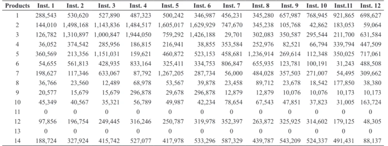
the maximum number of changeovers desired by the planners, so that each period has 4 sub-periods. Each instance comprises information about demand and initial inventory level for 14 products, which can be obtained by 19 different molding patterns, as Table 4 shows. More details about input data can be found in Martínez (2013).
Table 5 presents the results of the model after 3 hours. This table shows the incumbent solution after the limit time, the best upper bound, the gap provided by CPLEX, total elapsed time and the approximated time that the incumbent solution was found. As a general remark, the model was able to find feasible solutions for all the instances. However, its performance is not uniform for all of them, so that in some cases optimal solutions are found and in others the solutions have a high gap.
of the planning horizon. Meanwhile in the schedule provided by solving the model it is only 25.42%.
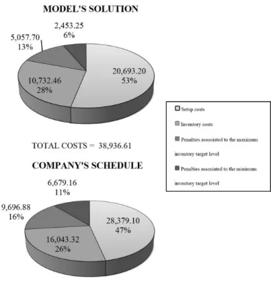
Some of the advantages of the model solution related to the costs involved are illustrated in Figure 2, which presents the total costs for each schedule.
Note that the schedule provided by the model’s solution incurred in approximately 35.96% less than the total costs of the company’s schedule. The main costs in the production process are the setup and the inventory holding costs, since they represent more than 70% of the total in both the schedules. Note that the setup costs in the model’s solution is approximately 27% less than the setup costs in the company’s schedule. In the same way inventory holding costs are also reduced about 33.1%.
Setup and inventory holding costs are lower in the model’s schedule, and penalties related to the inventory target levels were reduced as well. That was expected since the volumes of production and inventory levels are lower in the model’s solution than in the company’s schedule.
To analyze the performance of the GLSP model, a set of 12 instances was created based on real information provided by the company. These instances represent real data related to the number of products, possible molding patterns, production
Martínez, K. Y
. P
. et al.
656
Gest. Pr
od.
, São Carlos, v
. 23, n. 3, p. 649-660, 2016
Table 3. Production rates of the molding patterns (units per hour).
Products Molding patterns
1 2 3 4 5 6 7 8 9 10 11 12 13 14 15 16 17 18 19
1 8,791 0 0 0 0 0 0 0 0 0 7,326 5,862 0 0 7,326 5,862 0 0 4,395
2 0 8,791 0 0 0 0 0 0 0 0 0 0 0 0 0 0 0 0 0
3 0 0 8,791 0 0 0 0 0 4,395 0 0 0 0 0 0 0 0 0 0
4 0 0 0 8,791 0 0 0 0 0 0 0 0 0 0 0 0 0 0 0
5 0 0 0 0 8,791 0 0 0 0 7,326 0 0 0 0 0 0 0 0 0
6 0 0 0 0 0 8,791 0 0 0 0 0 0 0 0 0 0 0 0 0
7 0 0 0 0 0 0 8,791 4,395 0 0 0 0 7,326 5,862 0 0 7,326 5.862 0
8 0 0 0 0 0 0 0 3,295 0 0 0 0 0 0 0 0 0 0 0
9 0 0 0 0 0 0 0 0 3,295 0 0 0 0 0 0 0 0 0 0
10 0 0 0 0 0 0 0 0 0 1,465 0 0 0 0 0 0 0 0 0
11 0 0 0 0 0 0 0 0 0 0 0 0 1,465 2,929 0 0 0 0 0
12 0 0 0 0 0 0 0 0 0 0 1,465 2.929 0 0 0 0 0 0 1,465
13 0 0 0 0 0 0 0 0 0 0 0 0 0 0 0 0 1,465 2,929 0
Table 4. Initial inventory levels for the 12 instances.
Products Inst. 1 Inst. 2 Inst. 3 Inst. 4 Inst. 5 Inst. 6 Inst. 7 Inst. 8 Inst. 9 Inst. 10 Inst.11 Inst. 12
1 288,543 530,620 527,890 487,323 500,242 346,987 456,231 345,280 657,987 768,945 921,865 698,627
2 144,010 1,498,168 1,143,836 1,484,517 1,605,017 1,629,929 747,670 345,238 105,768 42,862 183,053 59,064
3 126,782 1,310,897 1,000,847 1,944,050 759,292 1,426,188 29,701 302,083 350,587 295,544 211,700 631,584
4 36,052 374,542 285,956 186,815 216,941 38,855 353,584 252,976 82,521 66,794 339,794 447,509
5 360,569 213,356 1,151,031 159,621 460,872 523,153 458,681 1,236,914 269,614 112,348 350,025 717,061
6 54,655 561,813 428,935 833,164 325,411 334,753 806,847 655,935 123,781 100,191 31,243 488,508
7 198,627 117,346 633,067 87,792 1,267,205 287,734 56,000 484,028 357,503 271,007 54,495 309,662
8 36,766 23,560 12,489 68,978 53,567 39,878 23,458 89,712 23,678 18,542 177,850 38,380
9 20,577 15,679 15,679 296,878 29,678 296,878 12,879 12,879 10,076 10,076 10,173 10,173
10 45,349 40,567 35,321 56,789 49,987 42,234 78,654 67,543 47,851 37,823 31,005 163,724
11 0 0 0 0 0 0 0 0 0 0 0 0
12 97,856 196,754 249,445 316,246 250,787 319,978 352,397 263,872 325,925 314,602 179,125 48,305
13 0 0 0 0 0 0 0 0 0 0 0 0
14 188,724 327,924 415,742 527,077 417,978 533,296 587,329 439,787 543,209 524,337 491,431 88,137
Table 5. Performance of the GLSP model.
Instance Incumbent/
optimal solution Lower bound Gap Elapsed time (s)
Time to ind
the incumbent/ optimal solution
(s)
1 71,568.38 26,872.47 62.45% 10,801.2 6,971.4
2 22,562.54 22,562.54 0% 118.7 90
3 19,325.65 19,325.66 0% 5,856.9 3,858
4 38,031.73 38,031.73 0% 433.5 301.2
5 23,882.86 23,882.86 0% 2,277.3 2,250
6 36,290.37 35,485.97 2.27% 10,801.5 4,980
7 35,718.47 35,445.11 0.77% 10,802.2 3,610.8
8 20,432.04 20,432.04 0% 1,591 390
9 31,554.20 29,783.99 5.61% 10,800.9 3,780
10 25,568.23 19,379.25 24.20% 10,801.4 6,024
11 20,476.83 20,476.83 0% 6,362 1,044
12 26,727.71 25,037.12 6.32% 10,801.1 1,022.4
Note than 50% of the instances were solved optimally in elapsed times which vary from 1 minute to 1 and a half hours. Among the instances which were not solved optimally, some solutions have a gap less than 6.5%. However, instances 1 and 10 were not easy to solve, since the incumbent solutions have gaps of 64.45% and 24.2%, respectively. Note in the last column of Table 5 that, on average, the model
gets the best solution in the irst minutes for most
of the instances. However, sometimes it spends a lot of time improving lower bounds.
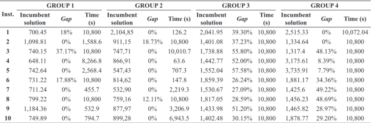
To make a better analysis of the model performance, some random instances were also tested. These data was generated based on Haase (1996) and Fleischmann & Meyr (1997) and comprise 4 different size groups of 10 instances. The characteristics of these random instances are presented in Table 6 and the results in Table 7.
Note that these instances are smaller in size than the real instances provided by the studied company.
Results show than the proposed model is able to provide feasible solutions for all the instances. However, optimal solutions only were found in the smaller size groups 1 and 2, which comprise only 2 machines, 6 molding patterns, 5 products, and 5 time periods. In the cases with more possible molding patterns, the performance of the model gets worse, since most of the instances have high gaps, which can exceed 50%.
It is worth mentioning that in the random instances the number of sub-periods for each period was determined as the number of possible molding patterns, i.e. S=N T* . Considering that in the real instances the number of sub-periods in each period was smaller, results suggest that the GLSP model has a better performance in those real instances, where
the number of sub-periods are deined based on the
Martínez, K. Y. P. et al.
658 Gest. Prod., São Carlos, v. 23, n. 3, p. 649-660, 2016
Some comparisons with real schedules for a particular instance were also presented in order to analyze the advantages of the model’s solutions.
These results evidenced how dificult it is to meet
the total demand without backlogs for the company’s planner. However, the model’s solution provided a schedule that met the full demand by using less capacity, lower setup time, setup costs, and inventory costs than the company’s schedule. Moreover, the model’s solution kept the inventory levels closer to the target levels. All these advantages are evidenced in a reduction of 27.08% of the setup costs, 33.10% of inventory costs, which consequently implied in a reduction of 36.96% in the total costs.
Acknowledgements
The authors thank the Graduate Program of Production Engineering from the Federal University of São Carlos – Sorocaba, Brazil (PPGEP-S), the Coordination for the Improvement of Higher Education Personnel (CAPES) for the grant and Sanovo Greenpack Embalagens do Brasil Ltda. for its collaboration in this research.
References
Almada-Lobo, B., Oliveira, J. F., & Carravilla, M. A. (2008). Production planning and scheduling in the glass container industry: AVNS approach. International
determined in advance. This parameter can be deined
either based on the experience of the planner or by preliminary computational experiments.
6 Concluding remarks and future
research
This paper studied the production planning and scheduling in molding packaging industry by particularly considering the production environment of a Brazilian company which produces packages for fruit and eggs. The planning decisions are related to the selection of molding patterns, how long they are used, and how they are sequenced. To represent those decisions we have proposed an optimization model based on the classical General Lot Sizing and Scheduling Problem (GLSP).
Results of the computational tests showed
that it is possible to ind feasible solutions for all
the instances by solving the model by CPLEX. For the real set of instances, 50% of them were solved optimally and approximately 33% have a gap of less than 10%. However, the performance
of the model is highly inluenced by the number of sub-periods deined for each period, which was deined based on the planners’ expertise for
the real set of instances. That suggests exploring alternative formulations that do not depend on
parameters deined in advance, which can inluence
the performance of the model.
Table 6. Characteristics of the random isntances.
Group # of instances # of molding patterns (N)
# of products (K)
# of time periods (T)
# of machines (L)
% expected capacity consumption (U)
1 10 6 4 5 2 80%
2 10 6 4 5 2 90%
3 10 10 6 5 2 80%
4 10 10 6 5 2 90%
Table 7. Results of the GLSP model for random instances.
Inst.
GROUP 1 GROUP 2 GROUP 3 GROUP 4
Incumbent solution Gap
Time (s)
Incumbent
solution Gap Time (s)
Incumbent solution Gap
Time (s)
Incumbent
Haase, K. (1996). Capacitated lot-sizing with sequence dependent setup costs. Operation Research Spectrum, 18(1), 51-59. http://dx.doi.org/10.1007/BF01539882.
Karimi, B., Ghomi, S. M. T. F., & Wilson, J. M. (2003). The capacitated lot sizing problem: a review of models and algorithms. Omega, 31(5), 365-378. http://dx.doi. org/10.1016/S0305-0483(03)00059-8.
Luche, J. R. D., & Morabito, R. (2005). Otimização na programação da produção de grãos eletrofundidos: um estudo de caso. Gestão & Produção, 12(1), 135-149.
Luche, J. R. D., Morabito, R., & Pureza, V. (2009). Combining process selection and lot sizing models for production scheduling of electrofused grains. Asia-Paciic journal of Operational Research, 26(3), 421-443.
Marinelli, F., Nenni, M. E., & Sforza, A. (2007). Capacitated lot sizing and scheduling with parallel machines and shared buffers: A case study in a packaging company.
Annals of Operations Research, 150(1), 177-192. http:// dx.doi.org/10.1007/s10479-006-0157-x.
Martínez, K. Y. P. (2013). Planejamento da produção na indústria de embalagens de polpa moldada (Dissertação de mestrado). Departamento de Engenharia de Produção – Sorocaba, Universidade Federal de São Carlos, Sorocaba.
Meyr, H. (2002). Simultaneous lotsizing and scheduling on parallel machines. European Journal of Operational Research, 139(2), 277-292. http://dx.doi.org/10.1016/ S0377-2217(01)00373-3.
Pattloch, M., Schmidt, G., & Kovalyov, M. Y. (2001). Heuristic algorithms for lotsize scheduling with application in the tobacco industry. Computers & Industrial Engineering, 39(3-4), 235-253. http://dx.doi. org/10.1016/S0360-8352(01)00004-3.
Pereira, P. Z., & Silva, R. P. (2010). Design de Embalagens e Sustentabilidade: uma análise sobre os métodos projetuais. Design & Tecnologia, 1(2), 29-43.
Silva, C., & Magalhaes, J. M. (2006). Heuristic lot size scheduling on unrelated parallel machines with applications in the textile industry. Computers & Industrial Engineering, 50(1-2), 76-89. http://dx.doi. org/10.1016/j.cie.2006.01.001.
Toledo, C. F. M., Arantes, M. D., & França, P. M. (2011). Tabu search to solve the synchronized and integrated two-level lot sizing and scheduling problem. Memorias de Annual Conference on Genetic and Evolutionary Computation, 13, 443-448.
Toledo, C. F. M., França, P. M., Morabito, R., & Kimms, A. (2007). Um modelo de otimização para o problema
Journal of Production Economics, 114(1), 363-375. http://dx.doi.org/10.1016/j.ijpe.2007.02.052.
Araujo, S. A., Arenales, M. N., & Clark, A. R. (2004). Dimensionamento de lotes e programação do forno numa fundição de pequeno porte. Gestão & Produção, 11(2), 165-176. http://dx.doi.org/10.1590/S0104-530X2004000200003.
Araujo, S. A., Arenales, M. N., & Clark, A. R. (2007). Joint rolling-horizon scheduling of materials processing and lot-sizing with sequence-dependent setups. Journal of Heuristics, 13(4), 337-358. http://dx.doi.org/10.1007/ s10732-007-9011-9.
Associação Brasileira de Embalagens – ABRE (2014).
Associação Brasileira de Embalagem apresenta balanço do setor. Recuperado em 14 de março de 2014, de www.abre.org.br
Augusto, D. B., Alem, D., & Toso, E. A. V. (2014). Planejamento agregado na indústria de nutrição animal sob incertezas. Produção. In press.
Clark, A., Morabito, R., & Toso, E. A. V. (2010). Production setup-sequencing and lot-sizing at an animal nutrition plant through ATSP subtour elimination and patching.
Journal of Scheduling, 13(2), 111-121. http://dx.doi. org/10.1007/s10951-009-0135-7.
Drexl, A., & Kimms, A. (1997). Lot sizing and scheduling - Survey and extensions. European Journal of Operational Research, 99(2), 221-235. http://dx.doi.org/10.1016/ S0377-2217(97)00030-1.
Ferreira, D., Clark, A. R., Almada-Lobo, B., & Morabito, R. (2012). Single-stage formulations for synchronised two-stage lot sizing and scheduling in soft drink production. International Journal of Production Economics, 136(2), 255-265. http://dx.doi.org/10.1016/j. ijpe.2011.11.028.
Ferreira, D., França, P. M., Kimms, A., Morabito, R., Rangel, S., & Toledo, C. F. M. (2008). Heuristic and meta-heuristics for lot sizing and scheduling in the soft drinks industry: a comparison study. Metaheuristics for Scheduling In Industrial and Manufacturing Applications Studies in Computational Intelligence, 128, 169-210. http://dx.doi.org/10.1007/978-3-540-78985-7_8.
Ferreira, D., Morabito, R., & Rangel, S. (2009). Solution approaches for the soft drink integrated production lot sizing and scheduling problem. European Journal of Operational Research, 196(2), 697-706. http://dx.doi. org/10.1016/j.ejor.2008.03.035.
Martínez, K. Y. P. et al.
660 Gest. Prod., São Carlos, v. 23, n. 3, p. 649-660, 2016
produção: estudo de caso numa fábrica de rações.
Gestão & Produção, 12(2), 203-217.
Toso, E. A. V., Morabito, R., & Clark, A. (2008). Combinação de abordagens GLSP e ATSP para o problema de dimensionamento e sequenciamento de lotes na produção de suplementos para nutrição animal.
Pesquisa Operacional, 28(3), 423-450. http://dx.doi. org/10.1590/S0101-74382008000300003.
Toso, E. A. V., Morabito, R., & Clark, A. R. (2009). Lot sizing and sequencing optimization at an animal-feed plant. Computers & Industrial Engineering, 57(3), 813-821. http://dx.doi.org/10.1016/j.cie.2009.02.011. integrado de dimensionamento de lotes e programação
da produção em fábrica de refrigerantes. Pesquisa operacional, 17(1), 155-186.
Toledo, C. F. M., França, P. M., Morabito, R., & Kimms, A. (2009). Multi-population genetic algorithm to solve the synchronized and integrated two-level lot sizing and scheduling problem. International Journal of Production Research, 47(11), 3097-3119. http://dx.doi. org/10.1080/00207540701675833.