Printed version ISSN 0001-3765 / Online version ISSN 1678-2690 http://dx.doi.org/10.1590/0001-3765201820170733
www.scielo.br/aabc | www.fb.com/aabcjournal
A weighted negative binomial Lindley distribution with applications to dispersed data
HASSAN S. BAKOUCH
Department of Mathematics, Faculty of Science, Tanta University, Tanta, 315277, Egypt Manuscript received on September 18, 2017; accepted for publication on January 5, 2018
ABSTRACT
A new discrete distribution is introduced. The distribution involves the negative binomial and size biased negative binomial distributions as sub-models among others and it is a weighted version of the two pa-rameter discrete Lindley distribution. The distribution has various interesting properties, such as bathtub shape hazard function along with increasing/decreasing hazard rate, positive skewness, symmetric behav-ior, and over- and under-dispersion. Moreover, it is self decomposable and infinitely divisible, which makes the proposed distribution well suited for count data modeling. Other properties are investigated, including probability generating function, ordinary moments, factorial moments, negative moments and character-ization. Estimation of the model parameters is investigated by the methods of moments and maximum likelihood, and a performance of the estimators is assessed by a simulation study. The credibility of the pro-posed distribution over the negative binomial, Poisson and generalized Poisson distributions is discussed based on some test statistics and four real data sets.
Key words:characterization, discrete distributions, Estimation, Vuong test statistic, mixture distributions, thunderstorms data.
INTRODUCTION
In observational studies it is observed that due to lack of well defined sampling frames for plant, human, insect, wildlife and fish populations, the scientists/ researchers cannot select sampling units with equal prability. As a result the recorded observations on individuals in these populations are biased unless every ob-servation is given an equal chance of being recorded. As such biased data arise in all disciplines of science, so statisticians and researchers have done their best to find out solutions for correction of the biases. In this regard, the weighted distribution theory gives a unified approach for modeling biased data, Fisher (1934), later on Rao (1985) and Patil (1991) studied it in a unified manner. Those pioneers have pointed out the situations in which the recorded observations cannot be considered as a random sample from the original distribution like non-experimental, non-replicated and non-random categories. This may be due to one or more reasons, such as non-observability of some events, damage caused to original observations and adop-tion of unequal probability sampling (see Jain et al. 2014). Patil and Rao (1977) stated that ”Although the
situations that involve weighted distributions seem to occur frequently in various fields, the underlying con-cept of weighted distributions as a major stochastic concon-cept does not seem to have been widely recognized”,
the same quote is applicable today but, unfortunately a rare work is seen on this topic.
In order to remove the biases and to obtain the suitable distribution, the researchers usually adopt the approach of weighted concept of biased observation which leads towards the development of a weighted distribution. For a non-negative integer valued random variable X, its probability mass function can be
defined asP(X =k) =p(k;θ),k∈N0={0,1, ...},where θ is a vector parameter, and letω(k) be a non negative function onN0,which does not need to be zero or one and may exceed unity but it should have a
finite expectation, i.e.,E(ω(X =k)) =∑∞
k=0ω(k)P(X=k)<∞. Suppose that when the event occurs, the weightω(k)is used to adjust the probability. Therefore, the recordkis thus the realization of count random
variableY which is a weighted version ofX and its probability mass function (pmf) is given by
P(Y =k) =pY(k;θ) =
w(k;ψ)P(X=k)
E(w(X;ψ)) ,k∈N0, (1)
where ω(k;ψ):≡ω(k) can depend on a parameterψ representing the recording mechanism, and it may also be connected to the underlying initial vector parameter θ. A detailed account of weight functions is available in Patil and Rao (1986). Some particular cases of the weight functions are the standard distributions with ω(k;ψ) =Constant,∀ k ∈ N0, the size-biased distributions with weightω(k;ψ) =k,∀k∈N0, the
popular COM-Poisson with weightω(k;ψ) = (k!)1−ψ,∀k∈N
0(see Balakrishnan 2014, pp. 511-512), Neel and Schull (1966) proposed the weighted Poisson distribution with a weight as Poisson distribution, i.e., ω(k;ψ) =ψ
ke−ψ
k! ,ψ>0,∀k∈ N0and binomial distribution with weight functionω(k;ψ) =1−(1−ψ) k, 0<ψ <1, ∀k∈ N0(see Kokonendji and Casany 2012).
In this paper, we construct a weighted version of the two parameter discrete Lindley distribution intro-duced by Hussain et al. (2016) by making use of the weight functionω(k;β) = β+kk−1. Construction and
motivations of the introduced distribution are outlined in the section below. Rest of the paper is organized as follows. The section ’Statistical Properties Of The WNBL Distribution’ gives several properties of the proposed distribution, such as probability generating function, moments, factorial moments, recurrence re-lation between moments and negative moments. In the section ’Parameter Estimation and Inference’, the estimation of the model parameters is investigated by the methods of moments and maximum likelihood, and performance of the estimators is assessed by a simulation study. A characterization for the distribution via the probability generating function is investigated with a discussion to self decomposability and infinite divisibility. Credibility of the proposed distribution over the negative binomial, Poisson and generalized Poisson distributions is also discussed based on some evaluation statistics and four real data sets. The last section gives the drawn conclusion.
THE PROPOSED DISTRIBUTION WITH MOTIVATIONS
Hussain et al. (2016) developed the two parameter discrete Lindley distribution with the pmf
P(X=k) =(1−p)
2(1+βk)pk
(1+βp−p) , (2)
Considering the weight functionω(k;β) = β+kk−1
and substituting it along with equation (2) into equation (1), we get
P(Y =k) =pk= 1
q+β2p
β+k−1
k
(1+βk)pkqβ+1, (3)
k∈N0,q=1−p,p∈(0,1)andβ≥0. Hereafter, the weighted version of the two parameter discrete Lindley distribution shall be denoted by the weighted negative binomial Lindley (WNBL) distribution. Now, we give some motivations for the proposed distribution.
Motivation 1. The pmf of the negative binomial (NB) distribution is given as
P(Y =k) =
β+k−1
k
pk(1−p)β
k,β∈N0andp∈(0,1), or equivalently
P(Y =k) =C
β+k−1
k
pk,
wherekdenotes the number of failures/success before theβthfailure/success,pis the probability of success andCis the normalization constant which equals(1−p)β. In the NB distribution, we repeat the number of Bernoulli trials in order to obtain a fixed number of successes, while if the number of failures/successes increases linearly on each trial then the probability of exactlykfailures/successes can be expressed as
P(Y =k) =A
β+k−1
k
(1+βk)pk,
whereA= qβ+1
q+β2p,β ∈N0⊆(0,∞),which is the pmf of the WNBL distribution.
Moreover, it can be noted that the probability function given by (2) is a generalized form of the NB with vector parameter(2,p)and also the discrete Lindley with vector parameter(1,p).
Motivation 2.
The binomial coefficient β+k−1 k
in the equation (3) represents the number of ways in which the fixed number of failures/successes are obtained when these failures/successes increase linearly on each trial.
Motivation 3.
It is also worth mentioning that the model given in equation (3) is recognized as a mixture of the NB distribution and the size biased negative binomial distribution (SBNB), that is,
pk=
q
q+pβ2NB(k;p,β) +
pβ2
q+pβ2SBNB(k−1;p,β). Motivation 4.
for such activities (see Sakamoto 1973). Therefore, we model such activities by introducing a weighted and mixed version of the negative binomial and Lindley distributions. The weighted distributions are important for the adjustment of probability of occurrences and removal of biasedness from the data, while the mixed distributions are usually used in heterogeneous and over-dispersed data sets. The proposed model not only overcomes the heterogeneity issue but also handles the over-dispersion because of its mixture representation which makes it better than the negative binomial, Poisson and generalized Poisson distributions.
Further motivations for the WNBL distribution are given in the next notes.
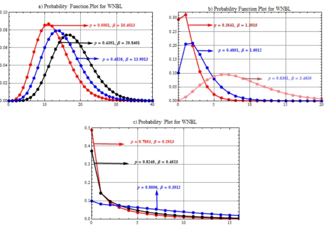
Figure 1 -Probability Graphs for the Indicated Values ofpandβ of WNBL.
Figure 1 portrays that the WNBL distribution shows symmetrical behavior when p<0.20 andβ in-creases. Whereas, for smallerβ and higherp,the distribution becomes positively skewed. The distribution
also exhibits bimodal and reverse J shapes.
Now, we give two prime measures of the distribution.
The survival and hazard rate functions of the WNBL distribution are
Sk =
(1−p)β+1pk(β) k (1+p(β2−1))xk!
×
(1+βk)2F1(β+k,1;k+1;p) +βp(β+k)2F1(β+k+
1,2;k+2;p)
(k+1)
, (4)
and
hk=
(1+βk)(k+1)
respectively. Where
2F1(a,b;c;z) = ∞
∑
n=0
(a)n(b)nzn (c)nn! ,
and(a)n=a(a+1)(a+2). . .(a+n−1), are the hypergeometric series function and the Pochhammer’s symbol, respectively, the series converges fora,b,c≥0and|z| ≤1.
Clearly
limk−→∞hk= (1−p)2,
therefore, the hazard rate function of the WNBL distribution is bounded above, which is an important property for the lifetime models.
Figure 2 -Hazard Function Graphs for the Indicated Values ofpandβof WNBL.
Figure 2 displays increasing, decreasing and bathtub shape (BTS) hazard functions. It is observed that the traditional statistical distributions, such as the Poisson, generalized Poisson and NB distributions, cannot be used efficiently in models of count data with many zeros. The Poisson distribution tends to under-estimate the number of zeros, while the NB may over-estimate zeros (see Saengthong and Bodhisuwan 2013). Al-though the traditional count models have generally increasing or decreasing failure rates yet unable to exhibit BTS hazard rates.
Being an over- and under-dispersed statistical model. iv) Being a self decomposable and infinitely divisible model. v) Being a characterizable function which is a milestone in model selection.
STATISTICAL PROPERTIES OF THE WNBL DISTRIBUTION
The recognition of any discrete probability distribution is usually based on its probability generating function (pgf). The following theorem gives the pgf of the WNBL distribution.
Proposition1:IfY ∼WNBL(p,β),then the pgf of the random variableY is expressed as
GY(t) =
(1+pt(β2
−1))qβ+1
(1+p(β2−1))(1−pt)β+1, (6)
where p∈(0,1)andβ≥0.
Proof:The pgf from the definition is expressed asGY(t) =∑∞x=0txP(Y =x). Using equation (3), we have
GY(t) =
qβ+1
1+p(β2−1)
∞
∑
x=0
β+x−1
x
(pt)x(1+βx)
,
which by simplification, equation (6) is obtained, which completes the proof.
Corollary 1:In equation (6), ift is replaced by et, we get the moment generating function (mgf) of the
WNBL distribution as
MY(t) =
(1+pet(β2
−1))qβ+1
(1+p(β2−1))(1−pet)β+1, (7)
where0<pet <1.
Therthderivatives of equation (7) with respect totatt=0yield the moments. In particular, forr=1,
we have
µ1′ =
βp(1+β+p(β2
−1)) (1−p)(1+p(β2−1)), forr=2,we have
µ2′ =
β(1+β)p(1−p(1−3β−(β−1)βp))
(1−p)2(1+p(β2−1)) ,
forr=3,we have
µ3′ =
β(1+β)p(1+p(−p+β(7+p(−1+6β+ (−1+β)βp)))) (1−p)3(1+p(β2−1))
and forr=4,we have
µ4′ = 1
(1−p)4(1+p(β2−1))×
{β(1+β)p(1+p(3+15β+ (−3+β(11+25β))p
+(−1+β(−2+β+10β2))p2+ (
−1+β)β3p3))
}.
Moreover, by definition, therthnon central moment can be expressed as
µr′= (1−p)
β+1 1+p(β2−1)
∞
∑
x=0
xr
β+x−1
x
Differentiating the equation above with respect top,we get dµ′
r
d p = −
∞
∑
x=0
xr
β+x−1
x
(1+βx)px{(β
2
−1)(1−p)β+1 (1+p(β2−1))2 +
(β+1)(1−p)β (1+p(β2−1))}
+ (1−p)
β+1 1+p(β2−1)
∞
∑
x=0
xr+1
β+x−1
x
(1+βx)px−1,
which by simplification yields the recurrence relation
µr′+1=p
dµr′
d p +
p(β+1)((β−1)(1−p) +1+p(β2
−1)) (1−p)(1+p(β2−1))2 µr′,
r=0,1, . . . ,µ0′ =1.
Similarly, by definition, therthcentral moment can be expressed as
µr=
(1−p)β+1 1+p(β2−1)
∞
∑
x=0
(x−βp(1+β+p(β
2
−1)) (1−p)(1+p(β2−1)))
r
β+x−1
x
(1+βx)px.
Differentiating the above equation with respect topand simplifying it, we get
µr+1+µ1′µr = p
dµr
d p +
pβ(β+1)(1−p)β(1+p(β−1))
(1+p(β2−1))2 µr
+r(β+1)((1+p(β 2
−1))2+ (β
−1)(1−p)2) (1−p)2(1+p(β2−1))2 µr−1,
r=1,2, . . . ,µ0′ =1.
OVER-AND UNDER-DISPERSION
In statistics, the phenomenon of over- and under-dispersion relative to the Poisson distribution is generally observed in count data and well known in statistical literature. There are various causes of such phenomenon, like heterogeneity and aggregation for over-dispersion and repulsion for under-dispersion although less fre-quent (see Kokonendji and Mizre 2005). In order to see the reflection of over- and under-dispersion pattern, the researchers usually take the support of the index of dispersion (ID) which is defined as variance-to-mean
ratio, which indicates the suitability of distribution in, under- or over-dispersed data sets. IfID>1(<1)the
distribution is over-dispersed (under-dispersed). The index of dispersion for the WNBL distribution is
ID= 1 1−p−
1
1−p+βp+
1
1+p(β2−1).
For indicating the dispersion pattern we first consider thatβ <1 which implies that β2
−1≤β−1. If β2
−1=−Candβ−1=−DthenIDcan be re expressed as
ID= 1 1−p−
1 1−pD+
1 1−pC,
sinceC>D,then1−pC<1−pDor 1−1pC−1−1pD >0. Therefore, the WNBL is an over-dispersed model for all values ofp. However, ifβ >1this implies thatβ2−1>β−1. Letβ2−1=Landβ−1=S,then IDcan be rewritten as
ID= 1 1−p−
1
1+pS+
1
1+pL.
OTHER MOMENTS MEASURES
The following theorems gives factorial moments and negative moments.
Theorem 1:IfY ∼WNBL(p,β), then therthdescending factorial moment ofY is given by
µ(′r)=(β)rp
r(1−p)−r(1+βr+ (β2
−1)p)
(1+p(β2−1)) , (8)
where p∈(0,1),β ≥0,r=0,1, . . . ,(a)n=a(a+1)(a+2). . .(a+n−1)andµ(′0)=1. Proof:Therth descending factorial moment for Y can be defined as µ′
(r)=E(Y(r)) =∑ ∞
x=0x(r)P(Y =x). Using the expressionx(r)=x(x−1). . .(x−r+1) =(x−x!r)!, we have
µ(′r)= (1−p)
β+1 (1+p(β2−1))
∞
∑
x=r
x! (x−r)!
β+x−1
x
(1+βx)px.
By using the binomial series(1−z)−a=∑∞
x=0
(a)nzn
n! , we obtain
µ(′r)=(1−p)
β+1(β+r
−1)!pr
(β−1)!(1+p(β2−1)){(1−p)−
(β+r)+β(r+ (r+1)(β+r)p+ (β+r)2(r+2)p2
2!. . .)}, hence, we get
µ(′r)= (1−p)−
r(β+r−1)!pr
(β−1)!(1+p(β2−1)){(1−p)−
(β+r)+ (1
−p)−(β+r+1)β(r+βp)}.
After some algebraic manipulation, the equation (8) is attained and it generates a recursive relation between
rand(r−1)descending factorial moments as
µ(′r){(1−p)(1+β(r−1) + (β2
−1)p)}={(β+r−1)p(1+βr+ (β2
−1)p)}µ(′r−1), (9)
wherer=1,2, . . . ,which completes the proof.
Theorem 2:IfY ∼WNBL(p,β), therthascending factorial moment ofY is given by
µ[′r]=βpr!(1−p)
β+1
(1+p(β2−1)){2F1(r+1,β+1; 2;p) +β2F1(r+1,β+1; 1;p)}, (10) where p∈(0,1),β ≥0,r=0,1, ...,µ[′0]=1− (1−p)β+1
(1+p(β2−1)).
Proof:Therth ascending factorial moment is defined asµ′
[r]=E((Y)r) =∑ ∞
x=0(x)rP(Y =x), this implies that
µ[′r]= (1−p)
β+1 (1+p(β2−1))
( ∞
∑
x=0
β+x−1
x
(x)rpx+β
∞
∑
x=0
β+x−1
x
x(x)rpx
)
.
By using the hypergeometric series function2F1(a,b;c;z) =∑∞n=0
(a)n(b)nzn
(c)nn! , we get the equation (10), where
∞
∑
x=0
β+x−1
x
(x)rpx=βr!p2F1(r+1,β+1; 2;p)
and
β
∞
∑
x=0
β+x−1
x
Thus the theorem is proved.
As it is known, the ordinary moments are generally helpful in estimating the unknown parameters. However, due to recent developments in inverse theory of the random variables, the negative moments are gaining momentum in life testing phenomena, estimation purposes and identifying the models. The negative moments are being used in irreversible damage to manufacturing materials due to damage process such as creep, corrosion, creep fracture, wear, shrinkage, aging and cracking (see Ahmad 2007). Therefore, the next theorem deals with the negative moments of the WNBL distribution.
Theorem 3:IfY∼WNBL(p,β),the first order negative moment ofY is given by
E (Y+a)−1
= (1−p)
β+1 (1+p(β2−1)){
1
a2F1(a,β;a+1;p) +
β2p
a+12F1(a+1,β+1;a+2;p)}, (11)
wherep∈(0,1),β≥0,a>0and2F1(a,b;c;z) =∑∞n=0
(a)n(b)nzn
(c)nn! .
Proof:By definition,E( 1 Y+a) =∑
∞
x=0 P(Y=x)
x+a , we have
E( 1
Y+a) =
(1−p)β+1 (1+p(β2−1))
∞
∑
x=0
β+x−1
x
(x+a)−1px(1+βx).
By simplification, we get the equation (11) where
∞
∑
x=0
β+x−1
x
px x+a =
1
a2F1(a,β;a+1;p)
and
∞
∑
x=0
β+x−1
x
xpx x+a =
βp
(a+1)2F1(a+1,β+1;a+2;p). This completes the proof.
Corollary 2:Thesthorder negative moment ofY ∼WNBL(p,β)can be expressed as
E (Y+a)−s
= (1−p)
β+1 (1+p(β2−1)){
1
as s+1Fs(a, ...,a,β;a+1, ...,a+1;p)
+ β
2p
(a+1)s s+1Fs(a+1, ...,a+1,β+1;a+2, ...,a+2;p)}, where
sFu(a1, ...,as;b1, ...,bu;z) =
∞
∑
n=0
(a1)n, ...,(as)nzn (b1)n, ...,(bu)nn!, the series converges fors=u+1and|z|<1.
PARAMETER ESTIMATION AND INFERENCE
MOMENTS METHOD
Let Y1,Y2, . . . ,Yn be a random sample drawn from the WNBL distribution with the observed values
x1,x2, . . . ,xn. Equating the first two sample moments, m′1=x¯= 1n∑ni=1xi andm′2= 1 n∑
n
i=1x2i,with their associated population moments
µ1′ =(β+1)p 1−p +
(β2
−1)p
1+p(β2−1) and
µ2′ =µ1′+((β+1)(β+2)p 2)
(1−p)2 +
2(β+1)(β2
−1)p2
(1−p)(1+p(β2−1)), then the MM estimators of the WNBL are obtained.
Alternatively, the MM estimators can also be obtained using the suggested approach by Khan et al. (1989) via minimizing the expression
S= (µ1′−m′1)2+ (µ2′−m′2)2,
with respect topandβ.Hence,
S = ((β+1)p
1−p +
(β2
−1)p
1+p(β2−1)−m′1) 2
+(m′1+
((β+1)(β+2)p2)
(1−p)2 +
2(β+1)(β2
−1)p2
(1−p)(1+p(β2−1))−m′2) 2
,
yields two equations which are not in closed form, so parameters are estimated using numerical optimization techniques via Mathematica 8 computational packages.
MAXIMUM LIKELIHOOD METHOD
IfY1,Y2, . . . ,Ynis a random sample drawn from the WNBL distribution with the observed valuesx1,x2, . . . ,xn, then we get the log-likelihood function
κp,β = ln(L(p;β)) = (β+1)nln(1−p)−nln((1+p(β
2
−1))) + n
∑
i=1
xilnp
+ n
∑
i=1
ln
β+xi−1
xi
+ n
∑
i=1
ln(1+βxi).
By partially differentiating both sides of the equation above with respect to pandβ and equating them to zero, we get theMLEsofpandβ,respectively, as
n(β+1) 1−p +
n(β2
−1) 1+p(β2−1) =
¯
x
p (12)
and
nln(1−p)− 2npβ 1+p(β2−1)+
n
∑
i=1
xi 1+βxi
+ n
∑
i=1
{ψ(0)(β+xi)
−ψ(0)(β)
}=0. (13)
Similarly, the second derivatives of the equations (12) and (13) with respect to pandβ,respectively, are
∂2κ p,β
∂p2 =−
n(β+1) (1−p)2 +
n(β2
−1)2 1+p(β2−1)−
∑ni=1xi
and ∂2κ
p,β
∂ β2 =
4np2β2 (1+p(β2−1))2−
n
∑
i=1
x2i
(1+βxi)2−
2np
1+p(β2−1)+ n
∑
i=1
n
ψ(1)(β+xi)
−ψ(1)(β)o .
Also, the second derivative of equation (12) with respect toβ or equation (13) with respect topyields
∂2κ p,β
∂ β ∂p =
2β(β2
−1)np
(1+p(β2−1))2−
n
1−p−
2βn
1+p(β2−1),
whereψ(n)(z) = dnψ(z)
dzn is the logarithmic derivative of the gamma function. The MLEs are computed using computational packages, such as Mathematica 7. In view of the regularity conditions (see Rohatgi and Saleh 2002, pp. 419), we observed that the MLEs of WNBL parameters satisfy such conditions, where i) The parametersp∈(0,1),β ∈(0,∞)are subset of the real line, ii)∂ κp,β
∂p ,
∂ κp,β
∂ β , ∂2κ
p,β
∂p2 , ∂2κ
p,β
∂ β2 , ∂2κ
p,β
∂p∂ β
exist for all values of pandβ, iii)E ∂ κ
p,β
∂p
=0,E ∂ κ
p,β
∂ β
=0,iv)−∞≤E ∂
2κ p,β
∂p2
!
≤0,−∞≤
E ∂
2κ p,β
∂ β2
!
≤0for all values ofpandβ.
Moreover, the MLEspˆandβˆof the WNBL distribution have an asymptotic bivariate normal distribution with vector mean (p,β) and variance-covariance matrix(I(p,β))−1, whereI(p,β)denotes the information
matrix given by
I((p,β)|p=pˆ
,β=βˆ) =
E(−∂
2κ
p,β ∂p2 ) E(
−∂2κ
p,β ∂p∂ β )
E(−∂
2κ
p,β ∂p∂ β ) E(
−∂2κ
p,β ∂ β2 )
, where
E(−∂
2κ p,β
∂p2 ) =
n(βˆ+1) (1−pˆ)2 −
n(βˆ2
−1)2 1+pˆ(βˆ2−1)+
nE(Y)
ˆ
p2 ,
E(−∂
2κ p,β
∂p∂ β ) =−
2 ˆβ(βˆ2
−1)npˆ (1+pˆ(βˆ2−1))2+
n
1−pˆ−
2 ˆβn
1+pˆ(βˆ2−1),
E(−∂
2κ p,β
∂ β2 ) =−
4npˆ2βˆ2
(1+pˆ(βˆ2−1))2+nE
Y2
(1+βˆY)2
!
+ 2npˆ
1+pˆ(βˆ2−1)−nE{ψ
(1)(βˆ+Y)−ψ(1)(βˆ)}
.
The expectations above can be obtained numerically.
SIMULATION SCHEME
As it is mentioned in the introduction that the WNBL(p,β)distribution can be viewed as a mixture of the
negative binomial, NB(p,β), and size biased negative binomial, SBNB(p,β), distributions. So, in order to
Algorithm: i) GenerateUi,i=1,2, ...,n,from the uniform distribution on the interval(0,1). ii) Generate
NBi,i=1,2, ...,n,from the negative binomial distribution NB(p,β)with supportk=0,1, . . .. iii)SetY1=
NBi. iv) Generate SBNBi,i=1,2, ...,n,from the size biased negative binomial distribution SBNB(p,β)
with supportk=1,2, . . .. v) SetY2=SBNBi. IfUi≤
1−p
(1+p(β2−1)), then setki=Y1,otherwise setki=Y2,
i=1,2, ...,n.
SIMULATION STUDY
In this section, we perform some numerical experiments to see how the estimates studied by using the above listed methods (MM and ML) as well as their asymptotic results for finite samples. All the numerical results are performed via Mathematica 8 using the random numbers generator code. We consider the following different model parameters. Model-I: β =0.0542,p =0.7487, Model-II: β =30.4389,p =0.0157 and
Model-III: β =5.2856,p=0.6398for both MMEs and MLEs. We consider the following sample sizes
n=20(small),50(moderate), and100,200,500(large). For each set of the model parameters and for each sample size, we compute the MMEs and MLEs of eachβ and p. We repeat this process1000times and compute the average bias and mean square error (MSE) for all replications in the relevant sample sizes. The results are reported in Tables I and II.
Discussion:Some notes are very clear from the simulation studies, such as the bias decreases as sample size increases for both MLEs and MMEs. Moreover, we conclude that the bias takes negative and positive signs, and it approaches to the value zero for both signs while the MSE decreases as the sample size increases.
CHARACTERIZATION
Characterization of probability functions is of importance to determine the exact probability distribution, which means that under certain conditions a family of distributions is the only one possessing a desig-nated property which will resolve the problem of model identification. Therefore, the next theorem gives characterization of the WNBL distribution.
Theorem 4:IfGY(t) =∑∞x=0xtP(Y =x)is the pgf of a certain distribution defined on the support{0,1,2, . . .} with parameters p∈(0,1),β ≥0, then
µ(′r){(1−p)(1+β(r−1) + (β2
−1)p)}={(β+r−1)p(1+βr+ (β2
−1)p)}µ(′r−1), (14)
forr=1,2, . . .withµ(′0)=1, holds if and only ifY has the WNBL distribution with pmf defined by equation
(3).
Proof:IfY has the WNBL distribution given by (3), then the equation (14) is satisfied.
On the other side, suppose the equation (9) holds, which yields descending factorial moments, hence forr=1andµ(′0)=1,we have
µ(′1)=(β)p(1−p)−
1(1+β+ (β2
−1)p)
(1+p(β2−1)) .
Forr=2andµ(′1)expressed in the above equation, we get
µ(′2)=(β)2p 2(1
−p)−2(1+2β+ (β2
−1)p)
TABLE I
Average Bias and MSE values of the MMEs from simulation of the WNBL distribution.
Parameter Sample Size Bias(βˆ) Bias(pˆ) MSE(βˆ) MSE(pˆ)
β =0.0542, p=0.7487
n=20 26.6700 -0.7485 742.1 0.5603
n=50 14.5694 -0.6458 411.023 0.4276
n=100 1.1141 -0.6022 1.4983 0.4265
n=200 0.9135 -0.5743 0.9130 0.3924
n=500 0.8783 -0.5517 0.8940 0.3822
β =30.4389, p=0.0157
n=20 139.4975 -0.7418 37071.8 0.5502
n=50 4.7926 -0.7071 23.0087 0.5001
n=100 4.4596 -0.6744 19.4900 0.4995
n=200 3.8780 -0.6688 18.8034 0.4872
n=500 2.8913 -0.6217 15.8204 0.4644
β =5.2856, p=0.6398
n=20 4.0410 -0.0942 12.6543 0.0125
n=50 3.6904 -0.0907 12.1628 0.0063
n=100 3.6522 -0.0890 9.8270 0.0058
n=200 3.3172 -0.0836 8.5084 0.0056
n=500 2.6516 -0.0798 8.2922 0.0047
Also, forr=3andµ(′2)expressed in the equation above, we obtain
µ(′3)=(β)3p 3(1
−p)−3(1+3β+ (β2
−1)p)
(1+p(β2−1)) ,
and so on. Since, factorial moment generating function is defined as
GY(1+t) =
∞
∑
r=0 µ(′r)t
r
r!, (15)
by substitutingµ(′0),µ(′1),µ(′2),µ(′3)and so on in equation (15) we get
GY(1+t) = 1+ βpt
(1−p)1!+
β2
pt
(1−p)(1+p(β2−1))1!
+β(β+1)p 2t2 (1−p)22! +
β2(β+1)p2t2 (1−p)2(1+p(β2−1))2!
+β(β+1)(β+2)p 3t3
(1−p)33! +
β2(β+1)(β+2)p3t3
TABLE II
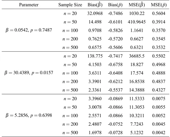
Average Bias and MSE values of the MLEs from simulation of the WNBL distribution.
Parameter Sample Size Bias(βˆ) Bias(pˆ) MSE(βˆ) MSE(pˆ)
β =0.0542,p=0.7487
n=20 32.0968 -0.7486 1030.22 0.5604
n=50 14.498 -0.6101 410.9645 0.3914
n=100 0.9708 -0.5826 1.1641 0.3570
n=200 0.7625 -0.5720 0.6627 0.3545
n=500 0.6575 -0.5606 0.6321 0.3532
β =30.4389, p=0.0157
n=20 138.775 -0.7417 36685.5 0.5502
n=50 4.1503 -0.6758 18.827 0.4968
n=100 3.6311 -0.6408 17.574 0.4888
n=200 3.3901 -0.6212 16.8538 0.4837
n=500 2.3361 -0.5537 14.3888 0.4327
β =5.2856,p=0.6398
n=20 3.3960 -0.0869 11.5333 0.0075
n=50 3.0078 -0.0866 11.3053 0.0055
n=100 2.5571 -0.0866 10.3211 0.0052
n=200 2.4807 -0.0752 7.7243 0.0045
n=500 1.6978 -0.0728 5.1232 0.0042
Hence,
GY(1+t) = 1+ βpt
(1−p)1!+
(β)2p2t2
(1−p)22!+
(β)3p3t3
(1−p)33!+. . .
+ β
2pt
(1−p)(1+p(β2−1))
1+(β+1)pt (1−p)1!+
(β+1)2p2t2
(1−p)22! +. . .
.
After some algebra, we get
GY(1+t) =
(1−p)β+1(1+p(1+t)(β2
−1)) (1−p(1+t))β+1(1+p(β2−1)). Replacing(1+t)bytwe have
GY(t) =
(1−p)β+1(1+pt(β2
−1)) (1−pt)β+1(1+p(β2−1)). By calculating thexthderivative ofGY(t)att=0,
P(Y =x) =
∂xG Y(t)
∂tx |t=0
DISCRETE ANALOGUES OF SELF-DECOMPOSABILITY
Definition 5.1 (α-thinning)LetXbe a non-negative integer-valued random variable and letα ∈[0,1], then theα-thinning ofXusing the Steutel and van Harn operator is defined by
α◦X:≡ X
∑
i=1
Zi,
whereZi (i=1,2, ...,X) are mutually independent Bernoulli random variables with P(Zi=1) =α and
P(Zi =0) =1−α. Additionally, the random variables Zi are independent of X. The pgfGα◦X(s) of the random variableα◦X is
Gα◦X(s) =GX(1−α+αs).
Definition 5.2 (Discrete Infinite divisibility)LetX be a non-negative integer-valued random variable, then X is said to be infinitely-divisible, for every non negative integern, ifX can be represented as a sum ofn
independent and identically distributed (i.i.d.) non-negative random variablesXn;i (i=1,2, ...,n), that is,
X ≡Xn,1+Xn,2+...+Xn,n, n=1,2,3, ... .
Note that the distributions ofXandXn;ido not necessarily have to be of the same family. Moreover, a random variableXis said to be discrete infinitely-divisible if the random variablesXn;ionly take non-negative integer values. A necessary condition for such random variableX to be well defined isP(X =0)>0(to exclude
the trivial case we assumeP(X=0)<1), see Steutal and van Harn (1979).
Definition 5.3 (Discrete self-decomposability)A non-negative integer-valued random variableXis said to be
discrete self-decomposable if for everyα∈[0,1],the random variableXcan be written asX≡α◦X+Xα,
where the random variablesα◦X andXα are independent, which in terms of the pgf can be expressed as
GX(s) =GX(1−α+αs)GXα(s),
whereGXα(s)is the pgf ofXα. We have noted that the distribution ofXαuniquely determines the distribution
ofX. Moreover, a discrete infinitely-divisible distribution is discrete self-decomposable.
By using the definitions above, the following propositions show that the WNBL distribution is a self decomposable and infinitely-divisible distribution.
Proposition 2:If X1,X2 and X3 are independent random variables such thatX1∼ Bernoulli( p(β 2
−1)
1+p(β2
−1)), X2∼NB(p,β)andX3∼Geo(1−p), thenY =X1+X2+X3has the WNBL(p,β)distribution.
Proof:SinceX1∼Bernoulli( p(β 2
−1)
1+p(β2−1)), its mgf is expressed asMX1(t) =
1+pet(β2
−1)
1+p(β2−1) . Similarly,X2andX3 having the mgfsMX2(t) = (1−p)
β
(1−pet)β andMX3(t) =
1−p
1−pet,respectively. SinceY =X1+X2+X3, hence the mgf ofY is
MY(t) =
1+pet(β2
−1) 1+p(β2−1)
(1−p)β (1−pet)β
1−p
1−pet, which is the mgf of the WNBL distribution. This completes the proof.
Proposition 3:IfYi∼WNBL(p,β)fori=1,2, ...n, are independent random variables, thenZ=Y1+Y2+
Y3. . .+Yn, and having the WNBL(n,p,β)distribution.
Proof:AsYi∼WNBL(p,β)fori=1,2, ...n, hence the mgf ofZ=Y1+Y2+Y3. . .+Ynis
MZ(t) = n
∏
i=1
MYi(t) =
(1+pet(β2
−1))n(1−p)n(β+1)
which gives the required proof. Note in the expression above
MZ(t) =MXB(t)MXNB(t),
where XB ∼ Binomial( p(β 2
−1)
1+p(β2−1),n) and XNB ∼ NB(p,n(β +1)), which shows the discrete
self-decomposability.
TEST STATISTICS WITH DATA APPLICATIONS
In this section, the credibility of the proposed model is checked via over- and under-dispersed count data sets. In this regard, for modeling over-dispersion phenomena, we have used three data sets: (i) The counts of European red mites on apple leaves, (ii) Accidents of 647 women working on H.E. shells during five weeks, (iii) The thunder storm activity at Cape Kennedy. While, for under-dispersion case the number of outbreaks of strikes in UK coal mining industries is used.All the data sets are modeled via the four probability models: WNBL, NB, Poisson (Poi) and Generalized Poisson (GP) distributions. Since NB distribution is the compounded mixture of gamma and Poisson distributions, so it is usually recommended for heterogeneity and over-dispersion, while the generalized Poisson distribution is a mixed and weighted version as well as a generalized form of Poisson distribution, therefore it is used to model over- and under-dispersed data sets. The probability functions of these models are given in the next table
The distribution formula Domain
PGP(Y =k) =(β(β+pk)
k−1e−β−pk)
k! k∈N0,p>
−1
β andβ >0
PNB(Y =k) = ((1−p)kpβ β+k−1
−1+β
) k∈N0,0<p<1andβ >0
PP(Y =k) =β
ke−β
k! k∈N0andβ >0
For comparison purposes, we have used seven goodness-of-fit statistics. The computation of these statis-tics is based on the MLEs which are computed by using Mathematica 7 computational package. These statistics include Log-Likelihood (l), Akaike information criterion (AIC), Bayesian information criterion
(BIC) and corrected Akaike information criterion (AICc), Kolmogrov Smirnov (KS) statistics andχ2 statis-tics with p−values. The formulae of such statistics areAIC =−2l(θ) +ˆ 2m,BIC =−2l(θ) +ˆ m ln(n),
AICc=AIC+2m(m+1)
n−m−1 ,KS=Max{
i
g−zi,zi− i−1
g }and χ
2= ∑gi=1
(oi−ei)2
ei , where
mdenotes the
number of parameters,l(θˆ)denotes the log-likelihood function evaluated at the MLEs,ndenotes the
num-ber of observations in a sample, g denotes the number of classes and oi, ei and zi denote the observed frequencies, expected frequencies and cumulative distribution function of theithclass, respectively. Vuong Test:The chi-square approximation to the distribution of the likelihood ratio test statistic is valid only for testing restrictions on the parameters of a statistical model, i.e.,H0andH1are nested hypotheses.
information criteria, like AIC and BIC as well as the Vuong test for non-nested models are useful. Vuong (1989) proposed a likelihood ratio-based statistic for testing the null hypothesis that the competing models are equally close to the true data generating process against the alternative that one model is closer. Let us consider two statistical models based on the probability mass functions fA(x;ξ)and fB(x;ζ)posses equal number of parameters. Define the likelihood ratio statistic for the model fA(x;ξ)against fB(x;ζ)as
LR(ξˆn,ζˆn) = G
∑
g=1
fgln
fA(x; ˆξn)
fB(x; ˆζn)
!
,
whereξˆ
nandζˆnare the maximum likelihood estimators in each model based onnnumber of observations(see Denuit et al. 2007),fgdenotes the observed frequency of thegthclass andGtotal number of classes . If both models are strictly non-nested then underH0we have the test statisticsZ=LR√(ξˆn,ζˆn)
nωˆn ∼
N (0,1), where
ˆ ωn=
1
G
G
∑
g=1
lnfA(xg; ˆξn) fB(xg; ˆζn)
!2
− 1
G
G
∑
g=1
lnfA(xg; ˆξn) fB(xg; ˆζn)
!2 .
In order to select an appropriate model, we usually construct the following hypothesis
H0;KL(fA(x;ξ)) =KL(fB(x;ζ)),
against
H1A;KL(fA(x;ξ))<KL(fB(x;ζ)),
i.e., the model A is defined to be better than model B if model A’sKLdistance to the truth is smaller than
that of model B, or
H1B;KL(fA(x;ξ))>KL(fB(x;ζ)).
That is, the model B is defined to be better than model A if model B’sKLdistance to the truth is smaller
than that of model A, whereKLdenotes the Kullback−Leibler distance measure, with corresponding critical
values. The decision is as follows.i)RejectH0whenZ>Zεin favor of A andii)RejectH0whenZ<−Zε
in favor of B, whereε denotes the level of significance.
DESCRIPTION OF THE DATA SETS WITH THEIR FITTING
In biological research, researchers are often concerned with animals and plants counts for each of set of equal units space and time. Among these sets of counts, some counts may perhaps be well fitted by the Poisson distribution where the equi-dispersion phenomenon in the data is observed. But in discrete data sets the two other dispersion cases are also observed. The over-dispersion generally arises when the events or organisms are aggregated, clustered or clumped in time and space, while the under-dispersion is due to more regular positioning than that produced by a Poisson mechanism (see Ross and Preece 1985). So, in the coming data applications we have also used the Vuong test for selecting a model which possesses the same number of parameters at significance level0.08, for this purpose we have compared the proposed model with the NB and GP, not with the Poisson distribution because the latter one is unsuitable for over- and under-dispersed data.
receiving the same spray treatment and the number of adult females counted on each leaf. These observa-tions given in Table III of the Appendix and were first recorded by Bliss and Fisher (1953), and later on were mentioned by Jain and Consul (1971). The summary statistics of these observations is provided in Table IV as given in Appendix which clearly indicates the over-dispersed nature of the data. In order to fit the competing models to this data set we have used the MLE estimates. The summary of test statistics is provided in Table V which depicts that the proposed model is the most suitable choice of such data with least loss of information. Moreover, the selection of a suitable non-nested model is also checked via Vuong test. The Vuong test statistics values along with p−valuefor comparison between WNBL-GP and WNBL-NB
are given asi)Z=−1.7548,p−value=0.0793,andii)Z=−1.7512,p−value=0.0799which clearly indicates the suitability of the proposed model by showing minimum p-value.
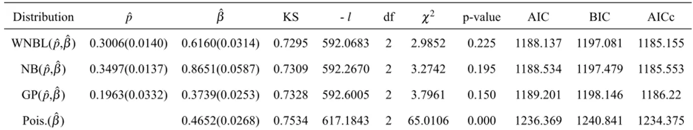
Accidents to 647 women working on H. E. shells during five weeks (Data II): Miss Broughton, Head Welfare Officer, and the various Welfare Supervisors were the first to provide this numerical data set to Industrial Fatigue Research Board in 1919 (see Greenwood and Woods, 1919). Later on Greenwood and Yule (1920) and Jain and Consul (1971) used it for analysis purpose. This data set is displayed at Table VI and its descriptive statistics are provided in Table VII which shows an over-dispersed behavior. The earlier mentioned test statistics indicate that the proposed model is the most suitable one according to all mentioned statistics with least loss of information behavior and the results are displayed in Table VIII as given in the Appendix. Furthermore, the Vuong test statistics values along with p−value for comparison between
WNBL-GP and WNBL-NB are given asi) Z=11.4348,p−value=0.0001,andii) Z=18.08284,p− value=0.0001which clearly indicates that the proposed model is better than the competing models.
Number of outbreaks of strikes in UK coal mining industries in four successive week periods during 1948-1959(Data III):This data set is given by Table IX and was analyzed by Castillo and Perez-Casany (1998), noting that they reported it from Kendall (1961). Later on a number of authors, like Ridout and Besbeas (2004), Chakraborty and Chakravarty (2012) and Alamatsaz and Dey (2016), studied it. Ta-ble X as given in the Appendix displays the descriptive statistics of this data set and indicates that it is under-dispersed. Further, comparison among the competing distributions is provided in Table XI which in-dicates that the proposed model is also an ideal model for under-dispersed data by showing not only the least Chi-Square test statistics but also minimum AIC, BIC and AICc, thus depicting that the model is the least loss of information model for under-dispersed data set too. Also, Vuong test statistics withp−values
for comparison between WNBL-GP and WNBL-NB are listed asi)Z=1.8540,p−value=0.0673,and ii)Z=4.4281,p−value=0.0001which again indicates the suitability of the proposed model.
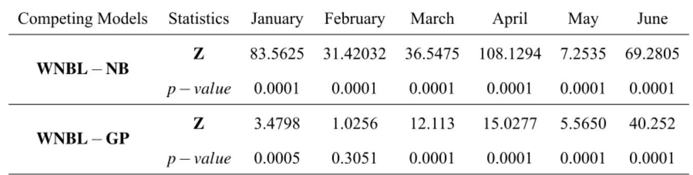
Thunderstorm Activity at Cape Kennedy(Data IV):One of the major problem that the meteorol-ogists usually faced is the forecasting of afternoon convective thunderstorm activity at the Cape Kennedy Florida. Usually thunderstorms are of primary concern in the design of launch vehicles, in the planning of space missions, and in launch operations at Cape Kennedy because of high winds, lightning hazard, and extreme turbulence associated with this atmospheric phenomenon. In thunderstorm activity, the occurrence of successive thunderstorm events (THEs) is often dependent process meaning that the occurrence of THEs indicates that the atmosphere is unstable and the environmental conditions are favorable for the formation of further thunderstorm activity. For more details on THEs, see Falls et al. (1971). Data set of thunderstorm ac-tivity at Cape Kennedy is displayed in Table XII at the Appendix. As for thunderstorm activities the Poisson distribution is not a proper choice, hence the proposed model is compared with the NB and GP distributions based on the expected frequencies,l, AIC,χ2andp
statistics of this data set are provided in the Tables XIII, XIV and XV. Vuong test statistics withp−values
are displayed in Tables XVI and XVII as given in Appendix, which clearly indicate the supremacy behavior of the proposed model over the competing distributions, except in February GP is recommended.
CONCLUSIONS
A new discrete model, named weighted negative binomial Lindley distribution, is proposed and its various properties are obtained involving generating functions, moments, recurrence relations between moments, random number generation, characterization, self-decomposability and infinite divisibility. Further, some applications of the model are studied. It is found that model is not only mathematically amenable but also recommended for many types of over- and under-dispersed count data sets. Moreover, the proposed model is also recommended for modeling the thunderstorms data and may help the scientists for proper planning of space missions and in launch operations at different stations in the presence of thunderstorms activities.
ACKNOWLEDGMENTS
The author express his thanks to Associate Editor of the mathematical sciences area and the two referees for careful reading of the paper and providing valuable comments. Special thanks to Professor Tassaddaq Kiani for his sincere help during the progress of this paper.
REFERENCES
AHMAD M. 2007. On the theory of inversion. Int J Stat Sci 6: 43-53.
ALAMATSAZ MH AND DEY S. 2016. Discrete generalized Rayleigh distribution. Pak J Stat 32(1): 1-20.
BALAKRISHNAN N. 2014. Methods and Applications of Statistics in Clinical Trials: Planning, Analysis and Inferential Methods. J Wiley & Sons, Inc.
BLISS CI AND FISHER RA. 1953. Fitting the negative binomial distribution to biological data. Biometrics 9(2): 176-200. CASTILLO I AND PEREZ-CASANY M. 1998. Weighted Poisson distributions for overdispersion and underdispersion situations.
Ann Inst Statist Math 50: 567-585.
CHAKRABORTY S AND CHAKRAVARTY D. 2012. Discrete gamma distributions: Properties and parameter estimations. Commun Statist Theor Meth 41: 3301-3324.
DENUIT M, MARCHAL X, PITREBOIS S AND WALHIN JF. 2007. Actuarial Modelling of Claim Counts Risk Classification Credibility and Bonus-Malus Systems. John Wiley.
FALLS L, WILLIFORD WO AND CARTER MC. 1971. Probability distributions for thunderstorm activity at Cape Kennedy, Florida. J Appl Meteorol 10: 97-104.
FISHER RA. 1934. The effects of methods of ascertainment upon the estimation of frequencies. Ann Eugenic 6: 13-25. GARMAN P. 1951. Original data on European red mite on apple leaves. Technical report. Report. Connecticut.
GREENWOOD M AND WOODS HM. 1919. The Incidence of Industrial Accidents upon Individuals with Special Ref-erence to Multiple Accidents. Industrials Fatigue Research Board Report URL https://ia802705.us.archive.org/29/items/ incidenceofindus00grea/incidenceofindus00grea.pdf. Online Address.
GREENWOOD M AND YULE GU. 1920. An inquiry into the nature of frequency distributions representative of multiple hap-penings with particular reference to the occurrence of multiple attacks of disease or of repeated accidents. J Roy Stat Soc 83: 255-279.
HUSSAIN T, ASLAM M AND AHMAD M. 2016. A two parameter discrete Lindley distribution. Rev Colomb Estad 39: 45-61. JAIN GC AND CONSUL PC. 1971. A generalized negative binomial distribution. SIAM J Appl Math 21: 501-5013.
JAIN K, SINGLA N AND GUPTA RD. 2014. A weighted version of gamma distribution. Discus Math Prob Stat 34: 89-111. KENDALL MG. 1961. Natural law in social sciences. J R Stat Soc Ser A 124: 1-19.
KOKONENDJI CC AND CASANY MP. 2012. A note on weighted count distributions. J Stat Theory Appl 11: 337-352.
KOKONENDJI CC AND MIZRE D. 2005. Overdispersion and Underdispersion Characterization of Weighted Poisson Distribution (Technical Report No. 0523) France LMA. Technical report.
NEEL JV AND SCHULL WJ. 1966. Human Heredity. Chicago: University of Chicago Press.
PATIL GP. 1991. Encountered data, statistical ecology, environmental statistics, and weighted distribution methods. Environmetrics 2: 377-423.
PATIL GP AND RAO CR. 1977. Weighted distributions: a survey of their application. In Krishnaiah PR (Ed.), Applications of Statistics, pp. 383-405. North Holland Publishing Company.
PATILL GP, RAO CR AND RATNAPARKHI M. 1986. On discrete weighted distribution and their use in model choice for observed data. Commun Statisit Theory Math 15: 907-918.
RAO CR. 1985. Weighted distributions arising out of methods of ascertainment. In Atkinson AC AND Fienberg SE (Eds.), A Celebration of Statistics Chapter 24. pp. 543-569. New York: Springer-Verlag.
RIDOUT MS AND BESBEAS P. 2004. An empirical model for under dispersed count data. Statist Model 4: 77-89.
ROHATGI VK AND SALEH AKE. 2002. An Introduction to probability and Statistics. Singapore: John Wiley and Sons (Asia) Pte Ltd.
ROSS GJS AND PREECE DA. 1985. The negative binomial distribution. The Statistician 34: 323-336.
SAENGTHONG P AND BODHISUWAN W. 2013. Negative binomial-crack (NB-CR) distribution. Int J Pure Appl Math 84: 213-230.
SAKAMOTO CM. 1973. Application of the Poisson and negative binomial models to thunderstorm and hail days probabilities in Nevada. Monthly Weather Review 101: 350-355.
STEUTEL FW AND VAN HARN K. 1979. Discrete analogues of self-decomposability and stability. Ann Prob 7: 893-899. VUONG QH. 1989. Likelihood ratio tests for model selection and non-nested hypotheses. Econometrica 57: 307-333.
APPENDIX
TABLE III
Counts of numbers of European red mites on apple leaves; data from Garman, 1951.
Count 0 1 2 3 4 5 6 7 Total
Observed frequency 70 38 17 10 9 3 2 1 150
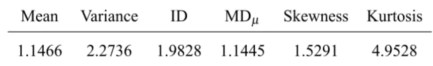
TABLE IV
Summary Statistics of data-I.
Mean Variance ID MDµ Skewness Kurtosis
TABLE V
Tests Summary for data set I.
Distribution pˆ βˆ KS -l df χ2 p-value AIC BIC AICc
WNBL(pˆ,βˆ) 0.2087(0.0154) 0.4770(0.0436) 0.5951 222.3063 3 2.3842 0.497 448.6126 454.6339 445.6926 NB(pˆ,βˆ) 0.5281(0.0275) 1.0245( 0.1051) 0.5979 222.4371 3 2.5147 0.473 448.8742 454.8955 445.9542 GP(pˆ,βˆ) 0.3209(0.0551) 0.7786(0.0796) 0.6019 222.7452 3 2.9475 0.400 449.4904 455.5117 446.5704 Pois.(βˆ) 1.1466(0.0874) 0.6408 242.8099 2 26.6513 0.000 487.6198 490.6304 485.6465
TABLE VI
Accidents to 647 women working on H. E. shells during 5 weeks.
Count 0 1 2 3 4 5 or more Total
Observed frequency 447 132 42 21 3 2 647
TABLE VII
Summary Statistics of data-II.
Mean Variance ID MDµ Skewness Kurtosis
0.4652 0.6919 1.4872 0.6428 2.1212 7.9209
TABLE VIII Tests Summary for data set II.
Distribution pˆ βˆ KS -l df χ2 p-value AIC BIC AICc
WNBL(pˆ,βˆ) 0.3006(0.0140) 0.6160(0.0314) 0.7295 592.0683 2 2.9852 0.225 1188.137 1197.081 1185.155 NB(pˆ,βˆ) 0.3497(0.0137) 0.8651(0.0587) 0.7309 592.2670 2 3.2742 0.195 1188.534 1197.479 1185.553 GP(pˆ,βˆ) 0.1963(0.0332) 0.3739(0.0253) 0.7328 592.6005 2 3.7961 0.150 1189.201 1198.146 1186.22 Pois.(βˆ) 0.4652(0.0268) 0.7534 617.1843 2 65.0106 0.000 1236.369 1240.841 1234.375
TABLE IX
Number of outbreaks of strikes in UK coal mining industries.
Count 0 1 2 3 4 Total
Observed frequency 46 76 24 9 1 156
TABLE X
Summary Statistics of Data-III.
Mean Variance ID MDµ Skewness Kurtosis
TABLE XI
Tests Summary for data set III.
Distribution pˆ βˆ KS -l df χ2 p-value AIC BIC AICc
WNBL(pˆ,βˆ) 0.0833(0.0077) 3.9294(0.2916) 0.5729 187.3976 1 1.1206 0.290 378.7952 384.8949 375.8721
NB(pˆ,βˆ) 0.0017(5.6903×10−06) 572.1488(45.9855) 0.5395 191.9723 1 9.4912 0.002 387.9446 394.0443 385.0215
GP(pˆ,βˆ) -0.1450(0.0403) 1.1376(0.0779) 0.5487 188.8228 1 4.5304 0.033 381.6456 387.7453 378.7225
Pois.(βˆ) 0.9936(0.0798) 0.5381 191.9362 2 9.4145 0.009 385.8724 388.9223 383.898
TABLE XII
Frequencies of the observed number of days that experience x TH’s at Cape Kennedy,Fla.,for 11-year period of Record January 1957 through December 1967.
x January February March April May June July August September October Nov. Dec. Spring Summer Fall 0 335 295 308 299 266 187 177 185 228 311 321 334 873 549 860
1 4 9 20 18 43 77 80 89 54 17 6 3 81 246 77
2 2 4 9 10 25 40 47 30 33 9 3 2 44 117 45
3 2 3 3 3 17 26 24 12 4 2 9 67 16
4 1 3 6 9 10 3 4 25 3
5 0 2 2 3 0 7
6 1 1 1 1
A
W
EIGHTED
NEGA
TIVE
BINOMIAL
LINDLEY
DISTRIBUTION
2639
x Jan. Feb. March April May June July Aug. Sep. Oct. Nov. Dec. Spring Summer Fall 0 334.99 294.92 307.72 298.62 265.09 185.42 173.55 184.55 225.47 310.66 320.97 333.98 871.38 543.54 857.62 1 4.63 10.34 22.56 21.67 49.00 83.09 91.84 87.20 65.33 20.41 6.95 4.197 93.70 262.13 93.87 2 0.98 2.92 6.64 6.16 16.57 36.22 43.18 39.67 24.21 6.06 1.48 1.43 28.96 119.04 29.91
3 1.06 2.42 2.16 6.25 15.14 18.98 17.26 9.25 2.25 0.65 10.69 51.37 11.41
4 0.96 2.45 6.14 8.00 7.28 3.55 4.24 21.43 4.67
5 0.98 2.44 3.28 3.01 1.74 8.73
6 0.39 0.96 0.73 3.49
Total 341 310 341 330 341 330 341 341 330 341 330 341 1012 1012 1001
LL(−l) 34.86 75.33 142.11 133.79 259.57 394.33 439.78 423.75 317.00 133.19 48.29 43.62 549.79 1258.98 560.87 ˆ
p 0.399 0.499 0.461 0.442 0.401 0.354 0.358 0.367 0.361 0.477 0.386 0.659 0.439 0.360 0.455
ˆ
β 0.034 0.066 0.141 0.144 0.731 0.815 0.740 0.526 0.123 0.053 0.019 0.019 0.204 0.760 0.200 Var(pˆ) 0.012 0.0051 0.0021 0.002 0.001 0.0003 0.0003 0.0003 0.0005 0.0023 0.0073 0.011 0.0005 0.0001 0.0005 Var(β)ˆ 0.0002 0.0002 0.0004 0.001 0.001 0.0019 0.0021 0.0018 0.0014 0.0004 0.0003 0.00003 0.0003 0.0006 0.0002
Cov(βˆ,pˆ) 0.0002 0.0012 0.001 0.001 0.001 0.0008 0.0008 0.0008 0.0009 0.0011 0.0015 0.0009 0.0003 0.0003 0.0003
Sk.((βˆ,pˆ) 161.49 85.3649 51.053 50.412 36.69 44.767 49.662 46.471 37.537 55.072 108.482 241.63 42.2 46.884 42.551
Kur.((βˆ,pˆ) 217.87 110.767 59.456 58.598 34.25 32.069 33.828 32.770 30.661 65.549 142.418 343.444 45.438 32.851 45.680
ID((βˆ,pˆ) 1.69 2.109 2.0204 1.946 1.860 1.640 1.6217 1.6728 1.7132 2.079 1.678 3.030 1.973 1.647 2.037
AIC 73.72 154.66 288.22 271.58 523.14 792.66 883.56 851.5 638 270.38 100.58 91.24 1103.58 2521.96 1125.74 χ2 0.027 0.032 1.173 3.250 5.504 2.392 4.538 5.745 5.559 3.306 0.038 0.083 9.80 7.90 11.18
df 1 1 2 2 3 4 4 4 3 3 2 1 4 5 3
p-value 0.869 0.858 0.556 0.197 0.138 0.664 0.338 0.219 0.135 0.347 0.981 0.773 0.044 0.162 0.011
An
Acad
Bras
Cienc
(2018)
HASSAN
S.
BAKOUCH
TABLE XIV Expected Frequencies,Log Likelihood,χ2,AIC and
p−valuesof the Observed number of days that experience x TH’s at Cape Kennedy,Fla.,from NB.
x Jan. Feb. March April May June July Aug. Sep. Oct. Nov. Dec. Spring Summer Fall 0 334.99 294.94 307.79 298.71 265.09 184.64 171.83 183.86 225.14 310.75 320.97 333.98 871.68 540.51 858.12 1 4.62 10.32 22.55 21.62 49.39 84.55 94.06 88.66 29.33 20.37 6.94 4.195 93.83 267.18 93.81 2 0.98 2.91 6.58 6.09 16.22 35.87 43.32 39.28 23.74 6.01 1.48 1.43 28.52 118.32 29.42 3 1.06 2.39 2.15 6.09 14.82 18.69 16.90 9.00 2.23 0.65 10.54 50.37 11.23
4 0.96 2.44 6.04 7.79 7.16 3.51 4.24 21.01 4.67
5 0.43 2.44 3.18 3.01 1.79 8.66
6 0.39 0.98 0.78 3.54
Total 341 310 341 330 341 330 341 341 330 341 330 341 1012 1012 1001 LL(−l) 34.86 75.34 142.17 133.86 259.78 394.59 440.18 423.95 317.57 133.26 48.29 43.62 550.14 1259.91 561.41
ˆ
p 0.412 0.528 0.510 0.492 0.471 0.391 0.374 0.404 0.422 0.524 0.405 0.659 0.500 0.391 0.518
ˆ
β 0.034 0.066 0.144 0.147 0.396 1.172 1.465 1.192 0.698 0.125 0.053 0.019 0.215 1.263 0.211 AIC 73.72 154.68 288.34 271.72 523.56 793.18 884.36 851.9 639.14 270.52 100.58 91.24 1104.28 2523.82 1126.82
χ2 0.028 0.035 1.232 3.347 6.008 2.888 5.428 5.967 6.429 3.307 0.039 0.084 10.38 9.51 11.87
df 1 1 2 2 3 4 4 4 3 3 2 1 4 5 3
p-value 0.867 0.852 0.540 0.188 0.111 0.577 0.246 0.202 0.093 0.347 0.981 0.772 0.034 0.090 0.008
Bras
Cienc
(2018)
90
A
W
EIGHTED
NEGA
TIVE
BINOMIAL
LINDLEY
DISTRIBUTION
2641
x Jan. Feb. March April May June July Aug. Sep. Oct. Nov. Dec. Spring Summer Fall 0 334.98 294.01 307.65 298.55 264.57 183.74 170.46 183.04 224.09 310.59 320.96 333.97 857.081 537.41 857.08 1 4.68 12.18 23.18 22.22 50.81 86.27 96.14 90.36 68.25 21.01 7.04 4.42 97.04 272.77 97.04 2 0.92 2.59 6.17 5.73 15.59 35.53 43.26 38.89 23.26 5.62 1.39 1.30 27.83 117.51 27.83 3 0.77 2.23 2.01 5.76 14.40 18.28 16.43 8.62 2.06 0.57 10.45 49.04 10.45
4 0.96 2.44 6.04 7.79 7.16 3.51 4.47 20.42 4.47
5 0.43 2.44 3.18 3.01 8.55 8.73
6 0.39 0.98 3.61 3.61
Total 341 310 341 330 341 330 341 341 330 341 330 341 1012 1012 1001 LL(−l) 34.94 75.88 142.57 134.35 260.26 394.98 440.81 424.34 318.36 133.79 48.41 43.92 551.65 1261.37 563.64
ˆ
p 0.241 0.245 0.312 0.297 0.279 0.221 0.207 0.231 0.239 0.323 0.236 0.453 0.303 0.221 0.316
ˆ
β 0.018 0.053 0.103 0.100 0.254 0.586 0.694 0.622 0.387 0.093 0.028 0.021 0.150 0.633 0.1552 AIC 73.88 155.76 289.14 272.7 524.52 793.96 885.62 852.68 640.72 271.58 100.82 91.84 1107.3 2526.74 1131.28
χ2 0.028 0.022 1.879 4.385 7.167 3.553 6.556 6.496 7.867 4.440 0.039 0.081 13.32 11.91 15.87
df 1 1 2 2 3 4 4 4 3 3 2 1 4 5 3
p-value 0.867 0.882 0.391 0.112 0.067 0.470 0.161 0.165 0.049 0.218 0.981 0.776 0.010 0.036 0.001
An
Acad
Bras
Cienc
(2018)
TABLE XVI Comparison via Vuong Test.
Competing Models Statistics January February March April May June
WNBL−NB
Z 83.5625 31.42032 36.5475 108.1294 7.2535 69.2805
p−value 0.0001 0.0001 0.0001 0.0001 0.0001 0.0001
WNBL−GP
Z 3.4798 1.0256 12.113 15.0277 5.5650 40.252
p−value 0.0005 0.3051 0.0001 0.0001 0.0001 0.0001
TABLE XVII Comparison via Vuong Test.
Competing Models Statistics July August September October November December
WNBL−NB
Z 90.2142 125.0967 26.7266 183.6862 1032.339 1838.215
p−value 0.0001 0.0001 0.0001 0.0001 0.0001 0.0001
WNBL−GP
Z 69.8226 54.8183 12.113 13.5131 6.1042 3.1211