ISSN 0104-6632 Printed in Brazil
www.abeq.org.br/bjche
Vol. 24, No. 04, pp. 523 - 533, October - December, 2007
Brazilian Journal
of Chemical
Engineering
EXPERIMENT AND NUMERICAL SIMULATION
ON THE PERFORMANCE OF A kW-SCALE
MOLTEN CARBONATE FUEL CELL STACK
L. J. Yu
1*, G. P. Ren
1X. M. Jiang
1, J. Q. Yuan
1, and G. Y. Cao
21
Institute of Thermal Energy Engineering, School of Mechanical Engineering, Phone: +(86) (21) 3420-6287, Fax: +(86) (21) 3420-5681,
Shanghai Jiao Tong University, Shanghai 200240, PR, China. E-mail: [email protected]
2
Institute of Fuel Cell, Shanghai Jiao Tong University, Shanghai 200030, PR, China
(Received: March 20, 2006 ; Accepted: November 13, 2006)
Abstract - A high-temperature molten carbonate fuel cell stack was studied experimentally and computationally. Experimental data for fuel cell temperature was obtained when the stack was running under given operational conditions. A 3-D CFD numerical model was set up and used to simulate the central fuel cell in the stack. It includes the mass, momentum and energy conservation equations, the ideal gas law and an empirical equation for cell voltage. The model was used to simulate the transient behavior of the fuel cell under the same operational conditions as those of the experiment. Simulation results show that the transient temperature and current and power densities reach their maximal values at the channel outlet. A comparison of the modeling results and the experimental data shows the good agreement.
Keywords: Molten carbonate fuel cell; Computational fluid dynamics; Numerical simulation; Three-dimension;
Transient model.
INTRODUCTION
Today fuel cells are considered environmentally friendly and high efficiency systems for the production of electricity, and worldwide research efforts have focused on improving this technology. Many projects, such as small-scale fuel cells for residential applications (Sammes and Boersma, 2000), the U.S. distributed generation fuel cell program (Williams et al., 2004), the MW-scale MCFC power plant (Ishikawa and Yasue, 2000) and fuel cell vehicles (Cacciola et al., 2001), have shown the prospects and great commercial value of fuel cells in the application fields of independent power sources and traffic. MCFCs have several advantages, e.g. high efficiency and cogeneration capability, over
low-temperature fuel cells because of their high operating temperature (650oC) (Kang et al., 2001). Sugiura et al. (2005) developed a performance diagnosis which enabled the simple and instantaneous determination of MCFC degradation factors. The performance diagnosis is helpful in developing MCFCs as a valuable technology. The commercial prospects of MCFCs were assessed by Dicks and Siddle (2000). It was anticipated that MCFC could have significant penetration into markets where its attributes, such as quality of power, low emissions and availability, give it a leading position in comparison with, for example, engine- and turbine-based power generation systems.
the MCFC stack greatly. The conductivity of the electrolyte in MCFCs increases with increasing temperature (Mangold, et al., 2004). There is about a one hundred degree temperature difference in MCFCs at maximum load. Big temperature gradient or high local temperature will lead to the corrosion of MCFC components and the evaporation of electrolyte. At the same time, the current density distribution is closely related to the temperature distribution (He and Chen, 1998; Koh et al., 2000). But experimental studies are expensive and the measurement of different variables is difficult, especially under transient conditions. Therefore, it is necessary to predict the temperature distribution and simulate MCFC stack performance numerically.
A lot of models for the MCFC can be found in literature, and most of them consider the steady state of the system under various parameters such as temperature distribution or pressure profile, electric efficiency or fuel usage (Yoshiba et al., 1998; Bosio et al., 1999; Koh et al., 2000). A good overview of some steady-state models can be found in Koh et al. (2001).
There are far fewer transient models. He and Chen (1998) developed a transient stack model using CFD in order to simulate the temperature profile, current density distribution and output of a MCFC stack. Lukas et al. (2002) developed a model for a single cell with indirect and direct internal reforming based on the assumption of concentrated parameters. However, the two above-mentioned models did not consider the effect of anode and cathode flow of gas mixture while analyzing the output of the MCFC.
Thus it is necessary to develop another transient
model based on physical phenomena. The three-dimensional, variational parameter, transient model presented takes into account the effect of anode and cathode flow of gas mixture to the output of a MCFC stack, which is necessary because of the variational gas mixture composition in the anode and cathode caused by mass transfer between them.
EXPERIMENT
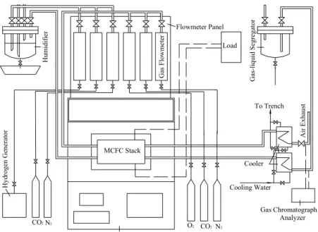
Fig. 1 schematically shows a kilowatt-scale MCFC stack testing station. Anode gas is composed of hydrogen (H2) and carbon dioxide (CO2). Anode
gas humidified by saturated water is preheated to 600 oC by a foreheater before it is fed into the MCFC stack. Cathode gas is composed of oxygen (O2),
carbon dioxide (CO2) and nitrogen (N2). The
electrolyte is a mixture of lithium carbonate (Li2CO3)
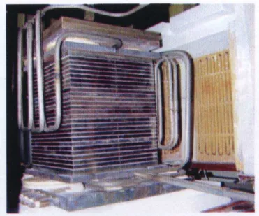
and potassium carbonate (K2CO3). Fig. 2 shows the
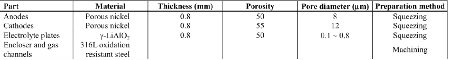
MCFC stack in the testing station. The stack has side-by-side coflow channels. Fig. 3 schematically shows a fuel cell in the stack and its components: bipolar plates which are composed of upper and bottom clapboards, a fuel cell unit which is composed of anode, cathode and electrolyte layer, and flow channels. Fuel and oxidant gas are fed into anode and cathode channels, respectively. Fuel gas oxidation and oxidant gas reduction are considered to occur only within the active catalyst layer. The test conditions and the geometric parameters of the fuel cells in the stack are listed in Table 1. The characteristics of the materials of the MCFC stack are listed in Table 2.
Electric Heater Controller
H
y
d
ro
g
en
G
en
er
at
o
r
N2 CO2
MCFC Stack
H
u
m
id
if
ie
r
A
ir
E
xha
us
t
Cooler
Cooling Water
CO2
O2 N2
To Trench
G
as
F
lo
w
m
et
er
G
as
-l
iqu
id
S
egr
ega
tor
Load Flowmeter Panel
Gas Chromatograph Analyzer
Figure 2: Kilowatt-scale MCFC stack
Cell unit Fuel gas
Oxidant gas
DC power Separator
Separator
Figure 3: Schematic diagram of a MCFC fuel cell
Table 1: Test conditions and geometric parameters of the experimental fuel cells
Gas-flow rate in the anode (l/min) 40
H2 and CO2 volume ratio in the anode 1:1
Humidifying temperature (oC) 60
H2, CO2 and water vapor volume ratio after humidification in the anode 2:2:1
Gas-flow rate in the cathode (l/min) 112.7
O2, CO2 and N2 volume ratio in the cathode 1:2:3.75
Percent of air utilized (%) 60
Li2CO3/K2CO3 mass ratio in the electrolyte 63:37
Number of fuel cells in the MCFC stack 30
Fuel cell area (m2) 0.24×0.14
Fuel cell height (m) 0.0042
Number of anode channels 34
Number of cathode channels 34
Channel length (m) 0.14
Channel width (m) 0.0037
Channel depth (m) 0.0016
Operating pressure (atm) 1
Table 2: MCFC stack materials and their characteristics
Part Material Thickness (mm) Porosity Pore diameter (µm) Preparation method
Anodes Porous nickel 0.8 50 8 Squeezing
Cathodes Porous nickel 0.8 55 12 Squeezing
Electrolyte plates γ-LiAlO2 0.8 50 0.1 ∼ 0.8 Squeezing
Encloser and gas channels
316L oxidation
resistant steel Machining
NUMERICAL MODEL
The units for all variables of the model equations are listed in the Nomenclature section, which is convenient for stating the model.
Model Assumptions
The present model assumes (1) Newtonian fluid and laminar flow; (2) ideal gas mixtures in the flow channels;
(3) he effect of the diffusion of carbonate ion
(CO32−) on the performance of the stack is neglected; (4) stable three-phase boundaries and water vapor in electrode capillaries;
(5) fluxes of hydrogen and oxygen along the diffusional direction equal to the consumption of hydrogen and oxygen in the electrochemical reaction in anode and cathode catalyst layers, respectively.
Assumption (3) is reasonable for the following two reasons: (a) the thickness of the electrolyte layer in the MCFC is 0.8 millimeter, which means the diffusional distance of carbonate the ions is very short; (b) the operating temperature of the MCFC is 650 oC and the electrolyte is in molten state, which makes the diffusional resistance of the carbonate ions in the electrolyte very small. Accordingly, assumption (3) won’t make simulations of the performance of the MCFC with a big error.
Electrochemical Reaction Process
Fig. 3 shows the physical model of a fuel cell in the stack. The fuel cell is a device that can convert chemical energy into electrical energy directly. Electricity and heat are generated during the electrochemical reaction of hydrogen and oxygen. The reaction can be expressed as
2 2 2
1
H O H O electricity heat 2
+ → + + (1)
The rate of the reaction and the heat source of reaction, based on work in the literature (Koh et al., 2000), are
i r
2F
= (2)
(
)
1Q= −∆ H r− iU δ (3)
where
(
)
H 240506 7.3835T
∆ = + (4)
The electric characteristics of the fuel cell can be obtained with a thermodynamical equation and experimental data. The thermodynamical equation (Koh et al., 2000) may be expressed as
2 2 2
2 2
H ,a O ,c CO ,c 0
eq
H O,a CO ,a
P P P
RT
E E ln
2F P P
= +
(5)
where
0 4
E =1.2723−2.7645 10× − T (6)
The fuel cell voltage, as represented by Koh et al. (2000) may be written as
cell eq ohm a c
U =E −i(R + η + η ) (7)
where Rohm is the ohmic resistance of the fuel cell
and related to the temperature of the fuel cell, ηis the impedance of electrode overpotential. The numerical results of polarization losses can be obtained from the work published by Koh et al. (2000).
4 ohm
1 1
R 0.5 10 exp[3016( )] T 923
−
2 2 2
9 0.42 0.17 1.0
a H CO H O
6435
2.27 10 exp( )P P P
T
− − − −
η = × (9)
2 2
10 0.43 0.09
c O CO
9298
7.505 10 exp( )P P T
− − −
η = × (10)
Governing Equations
a) Continuity Equation
Gases from anode and cathode in the stack do not mix during operation. The mass gain in anode channel flow is equal to the mass loss in cathode channel flow. The reason for equality is simply that for each mol of CO2 produced in the fuel flow, a mol
of CO2 is consumed in the oxidant flow due to
conservation of electric charge (Eqs.11, 12).
2
2 3 2 2
H +CO − →CO +H O+2e− (11)
2
2 2 3
1
CO O 2e CO
2
− −
+ + → (12)
The mass conservation equation for a control volume microunit whose location is fixed in the computational domain is
2 3
CO div( V) m
t −
∂ρ + ρ = ± ∂
G
(13)
where t is time, VJGis the velocity vector and 2
3 CO
m −
± is related to the local current density and the total area of electrochemical interface in the control volume.
b) Momentum Conservation Equation
The momentum conservation equation can be written, using Newton’s second law (F=ma) along the three directions of the coordinate axes for the control volume microunit, as
( V)
div( VV V) P
t
∂ ρ + ρ −µ∇ = −∇ ∂
JG JGJG JG
(14)
where µ is the viscosity of the gas mixture.
c) Energy Equations
The energy equation for the control volume microunit can be written, using gas mixture specific enthalpy (h) and temperature (T), based on the law of conservation of energy and Fourier’s law of heat conduction, as
h p
( h) h
div Vh S
t c
∂ ρ + ρ −λ∇ =
∂
G
(15)
where Sh is the heat source. In fuel gas flow, the heat
source is the heat generated in the water-gas shift reaction (Kim et al., 2002); in oxidant gas flow, it is zero.
The energy equation of the electrolyte layer can be written as
2
p h
( T)
c T S
t
∂ ρ − λ∇ =
∂ (16)
where Sh is the heat source in the electrolyte layer
and can be calculated using Eq. 3.
d) General Equation
A general equation can be abstracted from Eqs. 13-16 due to their comparability.
( )
div( V )) S
t φ φ
∂ ρφ + ρ φ −Γ ∇ φ = ∂
G
(17)
where φ is 1, h, and u, v, w in the continuity, energy, and momentum equations, respectively,
φ
Γ is the generalized diffusion coefficient, Sφis the source or sink.
There are seven unknown variables, i, u, v, w, P, T and ρ, in six equations, Eqs. 7, 13, 14 which is made of three equations and 15. Therefore, it is necessary to add an equation including P and ρ in order to make the model solvable.
f (P, c)
ρ = (18)
where P, for an ideal gas, is
where R is the molar gas constant.
As one of the physical characteristic parameters of the gas mixture in the stack, the generalized diffusion coefficient in Eq. (17) changes with the coordinates in the stack. And the reason is that the gas mixture components are different in different coordinates in the stack caused by electrochemical reaction. The variational generalized diffusion coefficient turns Eq. 17 into a group of variational coefficient equations.
Boundary Conditions
Boundary conditions at channel entries, such as gas mixture velocities, component concentrations and temperature and pressure at the channel outlet are specified and listed in Table 1. The two outer surfaces of the fuel cell are adiabatic because the computational domain of the fuel cell is located in the middle of the MCFC stack.
Numerical Procedures
The simulations in the study were carried out using computational fluid dynamics (Noriler, et al., 2004; Modenesi, et al., 2004). The coupled model equations, Eqs. 7 and 13-16, were solved numerically using the SIMPLEC algorithm for u, v, w, p, T, i and ρ. This approach was suggested by Van Doormaal and Raithby (1984), who modified the SIMPLE algorithm initiated by Patankar and Spalding (1972) and Patankar (1980). The block-correction technique (Prakash and Patankar, 1981; Patankar, 1981; Settari and Aziz, 1973) was used to accelerate the rate of convergence of the iterative solution. It was assumed that the reacting gases mixed well and the physical characteristics of the mixed gases changed with temperature. The coupled set of equations was solved simultaneously. The solution was considered to be convergent when the relative error of each physical variable between two consecutive iterations was less than 2×10⁻³. The SIMPLEC algorithm is as follows (Van Doormaal and Raithby, 1984):
(1) Assume an initial velocity distribution u0, v0, w0, based on which coefficient and constant term of the
momentum conservation equation, Eq. 14, are calculated;
(2) assume a pressure field P*;
(3) solve the momentum conservation equation, Eq. 14, getting u*, v*, w*;
(4) correct the pressure and velocity distributions using the continuity equation, Eq. 13, based on the requirement that the corrected velocity distributions, (u*+ u’), (v*+ v’) and (w*+ w’), which correspond to the corrected pressure, (P*+ P’), can satisfy Eq. (13);
(5) solve the energy equations, Eqs. 15 and 16, using the corrected velocity distributions, (u*+ u’), (v*+ v’) and (w*+ w’), getting temperature distribution, T; solve Eqs. 18, 19 and 5-10 using temperature distribution, T, and the corrected pressure, (P*+ P’), getting density and current distributions, ρ and i; (6) calculate the coefficient and constant term of Eq. 14 again, and use the corrected pressure distribution, (P*+ P’), as the initial value of the next iterative computation. The above steps continue iteratively till the convergent solution is obtained;
(7) steps (1-6) are concerning one time step, repeat the upper iterative computation in every time step, obtain the transient solution.
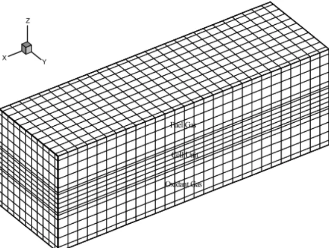
Computational Grids
X Y Z
Fuel Gas
Cell Unit
Oxidant Gas
Figure 4: Three-dimensional computational grids
RESULTS AND DISCUSSION
Based on the above model, the startup of the fuel cell is predicted and analyzed. It is assumed that the temperature of the fuel cell is preheated to 600 oC before startup. The testing conditions are listed in Table 1.
Comparison of the Calculated and Experimental Results
Fig. 5 compares the calculated temperature field and experimental data on the kilowatt-scale MCFC stack at the Institute of Fuel Cell, Shanghai Jiao Tong University, Shanghai, when the fuel cell was at steady state. The testing condition is the same as that for the simulations and is listed in Table 1. The temperature data were obtained using three thermoelectric couples that stuck to the current collector of the MCFC stack in the x direction. The calculated temperature field is at the cathode/current collector interface. Temperature in the former part increases sharply because of the heat generated in the
electrochemical reaction, while temperature in the back part is constant because of the increase in radiation loss. It can be observed in Fig. 5 that the modeling results compare well with experimental data, which means that the MCFC model can be used for more extensive simulations.
Calculated Results
Fig. 6 shows the startup temperature distributions at the cathode/current collector interface at times of 30, 60, 120, 360, 900, 1800, 3600 and 7200 s and steady state. The temperature of the stack increases sharply before 1800 s and appears to reach steady state after 7200 s.
Figs. 7 and 8 show the distributions of current and power densities in the MCFC stack, respectively. They are similar in shape to the steady-state distribution of temperature in Fig. 6. The increasing temperature in the direction of the x-axis makes local polarization loss decrease, which makes the current density and power density increase along the flow channel.
0.00 0.02 0.04 0.06 0.08 0.10 0.12 0.14
870 875 880 885 890 895 900 905 910 915 920 925
T
em
p
er
at
ur
e (
K
)
X (m)
Computed data Measured data
880 890 900 910 920
T
em
p
er
at
u
re
(K
)
0 0.05
0.1
X (m) 0
0.001 0.002
0.003 Y (m)
918.8 918.2
914.8 908.3 904.0 903.6
902.8 899.6 895.8 892.8 892.7
888.9 884.5 881.3 877.6
873.8
t=1800s t=3600s
t=900s
t=360s
t=7200s
t=120s t=60s
t=30s
t >>7200s
Figure 6: The start-up temperature distributions at the cathode/current collector interface
1200 1400 1600
C
u
rr
en
t
D
en
si
ty
(A
/m
2)
0 0.05
0.1
X (m) 0
0.001 0.002 0.003 Y (m)
X Z
Y
1645.9 1630.8 1596.0 1543.0 1495.4 1440.0 1392.5 1346.6 1297.4 1234.0
Figure 7: Current density distribution
900 1000 1100 1200 1300 1400
P
ow
er
D
en
si
ty
(W
/m
2)
0 0.05
0.1
X (m)
0 0.001 0.002 0.003 Y(m
)
X Z
Y
1426.5 1391.9 1316.6 1312.2 1283.0 1222.7 1146.1 1074.4 982.4
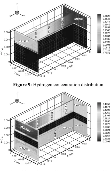
Figs. 9, 10 and 11 show the hydrogen, carbon dioxide and water vapor concentration distributions in the fuel cell, respectively. In the anode channel, the concentration of hydrogen decreases and the concentrations of carbon dioxide and water vapor increase during the reaction in Eq. 11; in the cathode channel, the concentration of
carbon dioxide decreases with the reaction in Eq. 12 and there are no hydrogen and water vapor.
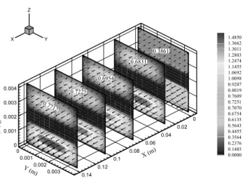
Fig. 12 shows the velocity distribution in the MCFC stack. The flow rate of the anode gas increases along the channel because of the mass transfer from cathode to anode.
0 0.001 0.002 0.003 0.004 Z (m ) 0 0.02 0.04 0.06 0.08 0.1 0.12 0.14
X (m)
0 0.001
0.002 0.003
Y (m)
0.224818 0 .2 5 9 8 5 4 0 .3 1 2 4 0 9 0 .3 6 2 0 4 4 0.39708 X Y Z 0.3825 0.3533 0.3241 0.2949 0.2657 0.2365 0.2073 0.1781 0.1489 0.1197 0.0905 0.0613 0.0321 0.0029
Figure 9: Hydrogen concentration distribution
0 0.001 0.002 0.003 0.004 Z (m ) 0 0.02 0.04 0.06 0.08 0.1 0.12 0.14
X (m)
0 0.001
0.002 0.003
Y (m)
0.47521 4 0.262371 0 .4 5 3 6 4 6 0 .4 3 0 8 2 4 0 .4 1 0 6 9 1 0.400702 0.2955 0.292933 0 .2 8 4 8 3 X Y Z 0.4752 0.4571 0.4398 0.4262 0.4107 0.3821 0.2955 0.2878 0.2786 0.2624 0.2623 0.1957 0.1025 0.0093
Figure 10: Carbon dioxide concentration distribution
0 0.001 0.002 0.003 0.004 Z (m ) 0 0.02 0.04 0.06 0.08 0.1 0.12 0.14
X (m)
0 0.001
0.002 0.003
Y (m)
0.298143 0 .2 7 6 2 2 1 0 .2 5 4 2 9 9 0 .2 2 7 9 9 2 0 .2 1 0 4 5 4 0.199493 X Y Z 0.2872 0.2653 0.2433 0.2214 0.1995 0.1776 0.1556 0.1337 0.1118 0.0899 0.0680 0.0460 0.0241 0.0022
0 0.001 0.002 0.003 0.004
Z
(m
)
0 0.02 0.04 0.06 0.08 0.1 0.12 0.14
X (m)
0 0.001
0.002 0.003 Y (m)
0.7225 0.6954
0.6831 0.3861
0.7712
X Y
Z
1.4850 1.3662 1.3011 1.2803 1.2474 1.1455 1.0692 1.0098 0.9207 0.8019 0.7609 0.7251 0.7070 0.6754 0.6135 0.5643 0.4455 0.3564 0.2376 0.1485 0.0000
Figure 12: Velocity distribution
CONCLUSIONS
A three-dimensional, variational parameter, transient model for a high-temperature MCFC stack was developed. The validity of the model was proved by comparison with measured temperature data obtained during the operation of the kW-Scale MCFC stack. The distributions of transient temperature on the cathode/current collector interface, current density, power density, hydrogen concentration, carbon dioxide concentration, water vapor concentration and velocity of the MCFC were obtained by solving the numerical model using the CFD method. The transient temperature and current and power densities reach their maximal values at the channel outlet.
The simulation results ofthe MCFC based on the model are consistent with the experimental data. Associated with a small-scale experimental study, the model can predict the performance of a large-scale MCFC numerically. This numerical model and the numerical method in the study will be helpful in designing large-scale MCFCs.
NOMENCLATURE
Latin Letters
c molar concentration, mol/m3 cp constant pressure specific
heat capacity,
J/kgK
Eeq reversible potential, V
E0 standard reversible potential, V F Faraday constant, 96500C/mol
h specific enthalpy, J/kg H molar enthalpy, J/mol
i current density, A/m2
m gas transportation flow rate, kg/m3s
P pressure, Pa
Q heat source, J/m3s
r reaction rate, mol/m2s R molar gas constant, 8.314J/molK Rohm ohmic resistance, Ωm2
Sh heat productivity, J/m3s
Sφ general heat source or sink
term
t time, s
T temperature, K
u, v, w
velocity components in x, y and z directions,
respectively,
m/s
VJG gas velocity vector, m/s
U electric voltage, V
x, y, z cell length, width and height, respectively,
m
Greek Letters
δ thickness, m
η impedance of electrode overpotential,
Ω m2
λ thermal conductivity, W/mK
µ kinematic viscosity, Pas
ρ density,
kg/m
3φ general variable
(-)
φ
Γ general effective transfer coefficient
Subscripts
a anode (-)
c cathode (-)
ACKNOWLEDGMENTS
This work was financially supported by the National Natural Science Foundation of China (No.50676058) and Shanghai Science and Technology Development (No. 993012003).
REFERENCES
Bosio, B., Costamagna, P. and Parodi, F., Modelling and Experimentation of Molten Carbonate Fuel Cell Reactors in a Scale-up Process, Chem. Eng. Sci., 54, No. 2907 (1999).
Cacciola, G., Antonucci, V. and Freni, S., Technology up Date and New Strategies on Fuel Cells, J. Power Sources, 100, No. 1-2, 67 (2001). Dicks, A. and Siddle, A., Assessment of Commercial
Prospects of Molten Carbonate Fuel Cells, J. Power Sources, 86, No. 1-2, 316 (2000).
He, W. and Chen, Q., Three-Dimensional Simulation of a Molten Carbonate Fuel Cell Stack Under Transient Conditions, J. Power Sources, 73, No. 2, 182 (1998).
Ishikawa, T. and Yasue, H., Start-up, Testing and Operation of 1000kW Class MCFC Power Plant, J. Power Sources, 86, No. 1-2, 145 (2000).
Kang, B.S., Koh, J.H. and Lim, H.C., Experimental Study on the Dynamic Characteristics of kW-Scale Molten Carbonate Fuel Cell Systems, J. Power Sources, 94, No. 1, 51 (2001).
Kim, M.H., Park, H.K., Chung, G.Y., Lim, H.C., Nam, S.W., Lim, T.H. and Hong, S.A., Effects of Water-Gas Shift Reaction on Simulated Performance of a Molten Carbonate Fuel Cell, J. Power Sources, 103, No. 2, 245 (2002).
Koh, J.H., Kang, B.S. and Lim, H.C., Effect of Various Stack Parameters on Temperature Rise in Molten Carbonate Fuel Cell Stack Operation, J. Power Sources, 91, No. 2, 161 (2000).
Koh, J.H., Kang, B.S. and Lim, H.C., Analysis of Temperature and Pressure Fields in Molten Carbonate Fuel Cell Stacks, AIChE J., 47, No. 9, 1941 (2001).
Lukas, M.D., Lee, K.Y. and Ghezel-Ayagh, H., Modelling and Cycling Control of Carbonate Fuel
Cell Power Plants, Control Eng. Pract., 10, No. 2, 197 (2002).
Mangold, M., Krasnyk, M. and Sundmacher, K., Nonlinear Analysis of Current Instabilities in High Temperature Fuel Cells, Chem. Eng. Sci., 59, No. 22-23, 4869 (2004).
Modenesi, K., Furlan, L.T., Tomaz, E., Guirardello, R. and Núnez, J.R., A CFD Model for Pollutant Dispersion in Rivers, Braz. J. Chem. Eng., 21, No. 4, 557 (2004).
Noriler, D., Vegini, A.A., Soares, C., Barros A.A.C., Meier, H.F. and Mori M., A New Role for Reduction in Pressure Drop in Cyclones using Computational Fluid Dynamics Techniques, Braz. J. Chem. Eng., 21, No. 1, 93 (2004).
Patankar, S.V., A Calculation Procedure for Two-Dimensional Elliptic Situations, Numer. Heat Transfer, 4, 409 (1981).
Patankar, S.V. and Spalding, D.B., A Calculation Procedure for Heat, Mass and Momentum Transfer in Three-Dimensional Parabolic Flows, Int. J. Heat Mass Transfer, 15, 1787 (1972). Patankar, S.V., Numerical Heat Transfer and Fluid
Flow. McGraw-Hill, New York (1980).
Prakash, C. and Patankar, S.V., Combined Free and Forced Convection in Vertical Tubes With Radial Internal Fins, ASME J. Heat Transfer, 103, 566 (1981).
Sammes, N.M. and Boersma, R., Small-Scale Fuel Cells for Residential Applications, J. Power Sources, 86, No. 2, 98 (2000).
Settari, A. and Aziz, K., A Generalization of the Additive Correction Method for the Iterative Solutions of Matrix Equation, SIAM J. Mumer. Anal., 10, 506 (1973).
Sugiura, K., Matsuoka, H. and Tanimoto, K., MCFC Performance Diagnosis by Using the Current-Pulse Method, J. Power Sources, 145, No. 2, 515 (2005).
Williams, M.C., Strakey, J.P. and Singhal, S.C., U.S. Distributed Generation Fuel Cell Program, J. Power Sources, 131, No. 1-2, 79 (2004).
Van Doormaal, J.P. and Raithby, G.D., Enhancements of the Simple Method Predicting Incompressible Fluid Flows, Numer. Heat Transfer, 7, 147 (1984).