On using the Hilbert transform for blind identification of systems with complex modes

Paper 824

On using the Hilbert transform for blind identification

of systems with complex modes

Jose Antunes(a), Philippe Piteau(b), Xavier Delaune(b), Laurent Borsoi(b), Vincent Debut(a,c) (a)

Centro de Ciências e Tecnologias Nucleares, Instituto Superior Técnico, Universidade de Lisboa, Estrada Nacional 10, Km 139.7, 2695-066 Bobadela LRS, Portugal,[email protected]

(b)

CEA-Saclay, DEN, DM2S, SEMT, Laboratoire d’Etudes de Dynamique, F-91191 Gif-sur-Yvette, France,[email protected],[email protected],[email protected]

(c)

Instituto de Etnomusicologia - Centro de Estudo de Música e Dança, Faculdade de Ciências Sociais e Humanas, Universidade Nova de Lisboa, Avenida de Berna, 26 C, 1069-061 Lisbon, Portugal,

[email protected]

Abstract

The modal identification of dynamical systems under operational conditions, when subjected to wide-band unmeasured excitations, is today a viable alternative to more traditional modal identification approaches based on processing sets of measured FRFs or impulse responses. Among current techniques for performing operational modal identification, the so-called blind identification methods are the subject of considerable investigation. In particular, the SOBI (Second-Order Blind Identification) method was found to be quite efficient. SOBI was originally developed for systems with normal modes. To address systems with complex modes, various extension approaches have been proposed, in particular: (a) Using a first-order state-space formulation for the system dynamics; (b) Building complex analytic signals from the measured responses using the Hilbert transform. In this paper we further explore the latter option, which is conceptually interesting while preserving the model order and size. Focus is on applicability of the SOBI technique for extracting the modal responses from analytic signals built from a set of vibratory responses. Aspects of the theoretical formulation for complex SOBI using the Hilbert transform are clarified and a convenient computational procedure for obtaining the complex cross-correlation response matrix is developed. We show that the correlation matrix of the analytic responses can be computed through a straightforward Hilbert transform of the standard real correlation matrix typically obtained from measurements. Then, based on numerical simulations of a physical multi-modal system subjected to distribute random excitation, we assert the quality of the identified modal matrix and modal responses extracted using both the standard and the complex SOBI techniques. To perform such analysis, a simple and feasible physical device is proposed, which enables controlled levels of the modeshapes complexity, without introducing significant modal damping even for strongly complex modes.

On using the Hilbert transform for blind identification

of systems with complex modes

1 Introduction

The modal identification of dynamical systems under operational conditions, when subjected to wide-band unmeasured excitations (turbulence, wind, waves, traffic), is today a viable alternative to more traditional modal identification approaches based on processing sets of measured FRFs or impulse responses. The advantages of operational modal identification are particularly obvious for systems difficult to excite, in particular civil structures such as bridges, towers or offshore platforms, but also for systems subjected to strong unmeasured force fields, such as turbulence-excited pipe systems. For most structures subjected to distributed wide-band random excitations, cross-correlation functions may be computed from the vibratory responses, which display the typical exponentially decreasing oscillatory behavior of impulse responses, sharing with them the essential dynamical properties of multi-modal systems.

This is the basis of NExT (Natural Excitation Technique) procedures, developed since the early 1990s, see [1]. Such correlation functions, or their corresponding spectra, may then be used for modal identification purposes, through various time-domain or frequency-domain identification techniques currently available. The books [2,3] offer recent reviews on the Operational Modal Analysis (OMA) and the techniques used for the modal identification of structures subjected to unmeasured excitations. Among approaches for performing operational modal identification, the so-called Blind Source Separation (BSS) methods are non-parametric modal extraction techniques which are currently subject of considerable investigation. A technique well adapted for performing operational modal identification is the Second-Order Blind Identification (SOBI) method, originally developed by Belouchrani et al. [4]. SOBI operates by extracting sources with different second-order temporal structure, therefore the identified system must not present degenerate modes, which would lead to modal responses with identical frequency content. SOBI is being increasingly used for the identification of real-life systems, see [3,5].

Then, illustrative real and complex modal identifications are presented, based on numerical time-domain simulations of a physical multi-mode system, with variable modal complexity, subjected to distribute random excitation. The illustrative computations presented are based on a specially designed rig, which enables achieving strong modal complexity with low modal damping. In the illustrative identifications produced we assert the quality of the identified modal matrix and modal responses, extracted using both the standard and the complex SOBI techniques, the later proving superior when addressing systems with high modal complexity.

2 Complex modal theory

2.1

Dynamics of non-proportionally damped systems

We start from the dynamical linear system:

( )

t



( )

t



( )

t



( )

t

My



Cy



Ky

f

(1)

where dissipation is modelled through a general damping matrix

C

, assumed symmetrical, but

not necessarily proportional as typically defined by:





1

1 1 2

0 ;

J _j

j j

α α  α 



  



C M K C M M K (2)

the latter being the general definition of proportionality derived by Caughey & Okelly [8]. Under the specific conditions (2), problem (1) leads to classical normal modes which are orthogonal

with respect to matrices M, K and

C

. Turning now to general dissipation conditions, equation

(1) may be written in equivalent state-space form, the first-order equation, see for instance [2,9]:

( )

t



( )

t



( )

t

Az



Bz

p

(3)

with the real composite matrices and vectors:

( ) ( )

; ; ( ) ;

( )

t t

t

t

       

_{ } _{ }  _{ } _{ }

       

C M K 0 y f

A B z p

M 0 0 -M y 0 (4)

Then, the modal formulation of (1) may be conveniently based on the complex eigenvalues and eigenvectors computed from the homogeneous form of (4), obtaining:



λnAB



ψn 0 (5)

with the modal pairs (over-bar designating the complex conjugate):

2

1 ; with

n n n R I

n n n n n n n

n n n n

i i

λ

ω ζ ω ζ

λ λ

   

      

   

   

φ φ

φ φ

φ φ

ψ (6)

2.2

Transfer functions and impulse responses

The transfer function matrix of system (1) is given as:



₂



1

( )ω  ω iω  

H M C K (7)

which, using results from complex analysis, may also be written as the modal summation of conjugate pairs:

1 ( )

N

n n

n i n i n

ω

ω λ ω λ



 

 



R R

where the residues are given by [9]:

2

; ; , 2 1

T T

n n n n

n n n n n n n

n n

a a m i

a a ω ζ

    

R φ φ R φ φ (9)

For systems with proportional damping matrix

C

display real modes φ φ φ_n  _n  _nR ϕ_n. For such

systems formulation (8) simplifies to:



2 2



1 ( ) 2 T N n n

n m_{n n} i _{n n}

ω

ω ω ωω ζ





 



H ϕ ϕ (10)

which is the classic transfer function when normal modes are used. The time-domain impulse responses

h

( )

t

are obtained by inverse Fourier transforming (8) or (10), hence:

1

( )

N

n n

n

nt nt

t

e

λ

e

λ









h

R

R

(11)

which, for normal modes, reduces to the usual result:



2



2 1

( ) sin 1

1 N

T

n n n n

n _{n n n}

n nt e t m t ω ζ ω ζ ω ζ     



h ϕ ϕ (12)

3 Modal responses and the Hilbert transform

3.1

Physical and modal responses

We now wish to formulate the impulse response in terms of the modal responses

q t

_n

( )

. Any

given column of the impulse matrix, denoted y in the following, is written:

1

( )

( )

( )

( )

( )

N

n n n n

n

t

q t

q t

t

t













y

φ

φ

φ

q

φ

q

(13)

with the complex modal responses given as:











2 2



2

1

( )

sin

1

cos

1

n n n n n n n

n n

n nt i t n nt

q t

 

c e

ω ζ

i e

ω ζ



c e

ω ζ

ω



ζ

t



i

ω



ζ

t

(14)

or ( ) R( ) I( )

n n n

q t q t iq t with:



2





2



( ) sin 1 ; ( ) cos 1

R I

n n n n n n n n

n nt n nt

q t c eω ζ ω ζ t q t  c eω ζ ω ζ t (15)

3.2

Use of the Hilbert Transform

The identification techniques addressed here concern vibrating systems with narrow-band modal responses, of which the impulse responses (13)-(15) are representative. The problem

now is, in presence of complex modes

φ φ



R



i

φ

I, how to relate the real and imaginary parts of such modal responses. Let us develop (13) as follows:

( ) ( )

( ) ( ) ( )

( ) ( )

R I

R I R I R R I I

R I

t i t

t i i t t

t i t

      _   _      q q

y q q

q q

and the physical response is real, as expected. One can see that, in presence of complex modes, there is an indeterminacy when attempting to extract the complex modal responses

( )

t



R

( )

t



i

I

( )

t

q

q

q

from the real physical responses y( )t . Finding a manner to overcome this

fundamental difficulty is at the root of the developments that follow. Let us build the analytic signal counterpart of equation (13), by use of the Hilbert Transform:





( )

ˆ( ) ( )

( )

PV

t t d

t

τ _τ

π τ

 



 





y

y H y (17)

where

PV

stands for the Cauchy principal value, as the integrated function displays a singularity at

τ



t

, see [10]. The Hilbert transform being a linear operator, each term of a modal series may be transformed independently. Then:





ˆ ˆ

ˆ( )t  ( )t  R R( )t  I I( )t

y

H

y φ q φ q (18)

hence the complex analytic signal:



 

ˆ ˆ



ˆ

( )t i ( )t  R R( )t  I I( )t i R R( )t  I I( )t

y y φ q φ q φ q φ q (19)

Looking at the expressions for the modal responses q t_n( )q t_nR( )iq t_nI( ), equations (15), these

naturally consist on oscillatory functions multiplied by exponential decreasing functions. A difficulty of performing the Hilbert transforms of (15) is the that these are not readily available for function products. Nevertheless, these may be approximated and we obtain the Hilbert transform q tˆ_n( )q tˆ_nR( )iq tˆ_nI( ) with:



2





2



ˆnR( ) n cos n 1 n ; ˆnI( ) n sin n 1 n

n nt n nt

q t  c eω ζ ω ζ t q t  c eω ζ ω ζ t (20)

Then, by comparing results (15) and (20), one concludes that:

ˆ

ˆ

( )

( ) ;

( )

( )

I R I R

t



t

t

 

t

q

q

q

q

(21)

so that formulation (19) based on the analytic responses simplifies to:



ˆ

 

ˆ

 



ˆ



ˆ

( )t i t( ) R R( )t  I R( )t i R R( )t  I R( )t  Ri I R( )t i R( )t

y y φ q φ q φ q φ q φ φ q q (22)

or, using notation y( )t y( )t iyˆ( )t and

q



R

( )

t



q

R

( )

t



i

q

ˆ

R

( )

t

for the analytic signals:

( )

t



R

( )

t

y



φ

q



(23)

Formulation (22) was proposed by McNeill [11], although fewer details were reported. The essential merit of this approach, when compared with the basic formulation (16), is that the

indeterminacy on

q

I

( )

t

disappears from the identification problem, as now only two vectors of analytic signals are equated, whose imaginary components are directly related to the real components through the Hilbert transform.

4 SOBI identification

4.1

Systems with real modes

Whatever the excitation, the physical responses

y t

_r

( )

at

r



1, 2,



,

R

measurement locations

are related to the modal responses

q t

_n

( )

through modal superposition. For real modes

ϕ

_n the

classic expression applies:

1 2

( )

t



( ) with

t





r

, , ,

r _Nr



_

y

ϕ

q

ϕ ϕ ϕ

_

ϕ

(24)

where the modeshape vectors ϕnr are taken at the r1, 2,,R measurement locations. Then,

from (24), one easily obtains the matrix relationship between the physical response cross-correlations and the modal response cross-correlations:

( )τ E_ (tτ) ( )t T_E_ (tτ) ( )t T T_ E_ (tτ) ( )tT_ T ( )τ T

yy qq

R y y ϕq q ϕ ϕ q q ϕ ϕR ϕ (25)

Moreover, by Fourier transforming (25), a similar relation is obtained for the response spectra:

( )ω  ( )ω T

yy qq

S ϕS ϕ (26)

Equations (25) and (26) are quite general, as the specificities of different excitations will be reflected on the system modal responses.

When the system modeshapes are unknown, the identification problem falls in the realm of the so-called blind identification, which aims the simultaneous extraction of both the modeshapes ϕ

and modal responses encapsulated in S_qq( )ω and R_qq( )τ . For such purpose, the Second

Order Blind Identification (SOBI) technique is recognized as quite effective. SOBI operates on second-order time-domain functions, using the correlation matrix R_yy( )τ of the measured

responses. Simultaneous diagonalization is usually applied to the modified correlation matrix

( )

τ

ww

R

, computed from data modified through a whitening matrix W. Then, the problem to

solve is finding the unitary matrix

U

which minimizes the off-terms in the matrix products

( ) T

k τ ww

U R U, with k 1, 2, ...,K :





2

1

m in off ( )

K k

T

k

J τ







_{w w}

U U R U

( ) (27)

The mixing matrix ϕ is deduced from the unitary matrix

U

identified through (27), using the

inverse transformation

ϕ =

W U

1 .

4.2

Systems with complex modes

We now address the more difficult question of using SOBI for systems with complex modes. Recalling the basic relation (23), we now have:

1 2

( )

t



R

( ) with

t





r

, , ,

r _Nr



_

y



φ

q



φ φ φ



φ

(28)

where the complex modeshape vectors φnr φnRriφnIr are taken at the r1, 2,,R

measurement locations. Also, we recall that the physical and the modal response vectors are

formulate the cross-correlations of the physical and the modal responses, formulated in terms of their analytic signals. We obtain from (28):

( )τ _ ( )τ H

yy qq

R_{ } φR_{ } φ (29)

with R_{yy }( )τ  E_y(tτ) ( )y t H_ and R_{qq }( )τ  E_qR(tτ)qR( )t H_. The SOBI diagonalization of complex matrices has been the subject of recent research. In the present paper the effective technique developped by Tichavsky & Yeredor [12] will be used. In the same manner each real modeshape ϕnr is identified up to an arbitrary real constant

r

n, each complex modeshape

r Rr Ir

n  n i n

φ φ φ is identified up to an arbitrary complex constant c_n c_nR ic_nI. The modal scaling constants

c

_n also impose a suitable rotation in the complex plane, so that the real component of

normalized complex modeshape be as dominant as possible.

4.3

Simplified computation of the complex correlation matrix

The cross-correlations in (29) are easily computed as:

0

( ) ( ) ( ) , , 1, 2, ,

yy

rs r s

R τ y t τ y t dt r s R





_

 

 

   (30)

or, developing:

ˆ ˆ

ˆ ˆ

( ) ( ) ( ) ( ) ( ) ( ) w ith

( ) ( ) ( )

R yy yy yy

yy R yy I yy rs rs rs

rs rs rs I yy yy yy

rs rs rs

R R R

R R i R

R R R

τ τ τ

τ τ τ

τ τ τ

  

  _

 



 

     

  (31)

If one has direct access to the time-domain response measurements

y t

_r

( )

, equations (30) or

(31) may be easily applied, because the analytic signals can be computed from the measurements. However, it often happens that the raw response measurements are not recorded or have been lost, so that one only has access to statistical quantities such as the correlation or spectral functions. Under those circumstances, it becomes impossible to compute the cross-correlations of the analytic signals. The problem then becomes, given the basic

measurement correlations yy( )

rs

R τ , if it is possible - and how - to estimate the real and imaginary

components of Rrsyy( )τ  RRrsyy( )τ i RI rsyy( )τ

     

. It may be shown that:





_____________________



ˆ ˆ_{( )} 1 _{sgn( ) ( ) sgn( ) ( )} 1 _{( ) ( ) ( )}

yy yy

rs r s r s rs

S i y i y y y S

T T

ω   ω ω  ω ω  ω ω  ω (32)

hence:

ˆ ˆ_{( ) ( )}

yy yy

rs rs

R τ R τ (33)

Turning to the terms in the imaginary part IR_rsyy ( )τ , we have for the first one:

ˆ _{( )} 1 _{ˆ ( ) ( ) sgn( ) ( ) ( ) ˆ ( )}

yy yy yy yy

rs r s rs rs rs

S y y i S S S

T

ω  ω ω   ω ω H _ ω _ ω ₍₃₄₎

hence:

ˆ

_ˆ

( )

( )

yy yy

rs rs

R

τ



R

τ

(35)

ˆ_{( )} 1 _{( )ˆ ( ) sgn( ) ( ) ( ) ˆ ( )}

yy yy yy yy

rs r s rs rs rs

S y y i S S S

T

ω  ω ω  ω ω  H _ ω _  ω (36)

hence:

ˆ

_{( )}

_ˆ

_{( )}

yy yy

rs rs

R

τ

 

R

τ

(37)

Finally, we obtain from (31), with (33), (35) and (37):







ˆ



( )

2

( )

( )

2

( )

( )

yy yy yy yy yy

rs rs rs rs rs

R



τ



R

τ



i

H

_



R

τ



_



R

τ



i R

τ

(38)

which is the essential result of this section, to the authors best knowledge still absent from the literature. It states that, given the correlation matrix R_rsyy( )τ of a set of response measurements,

one can easily deduce the correlation matrix of their complex analytic counterparts through the Hilbert transform of R_rsyy( )τ . Beyond being much simpler than the direct result (31), the derived

equation (38) is of considerable practical value, as it allows for complex modal identification even when the original time-domain response data is not available for post-processing.

5 Illustrative results

5.1

Computed system

A simple continuous system under different conditions will illustrate the techniques presented. It consists on a pinned-pinned beam with L 1.0 m and modal frequencies f_n n f2 ₁, with

1

10 Hz

f



, modal masses

m

_n



0.5 Kg

and modal damping

ζ

_n



1 %

for all modes, of the form

( )x sin(n x L/ )

ϕ  π . The beam is excited by a set of 29 regularly spaced uncorrelated

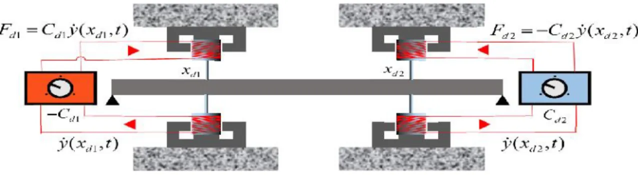
point-forces, delivering banded white-noise excitations in the range 0 ~ 1000 Hz, each one with a RMS amplitude of 1 N. This basic system has uniformly distributed dissipation and therefore normal (real) modes. In order to obtain a system with strongly complex modes, localized

dissipation may be applied as shown in Figure 1(a) where a damper

C

_d is attached to the beam

at location

x

_d



0.75

L

.

Figure 1: Systems with complex modes: (a) Using a damper

d

C at location 0.75

d

x  L; (b) Using a negative damper

1

d

C

 at location

1 0.25

d

x  L and a normal damper

2

d

C at location

2 0.75

d

x  L.

However, as might be expected, modal damping at the lower modal frequencies severely

undesirable feature, we propose to use the modified system sketched in Figure 1(b), which includes two symmetrical dampers



C

_d1 and

C

_d2 located respectively at

x

_d1



0.25

L

and

2

0.75

d

x



L

, the first one being destabilizer and the other being dissipative.

Figure 2: Practical test rig for the near-conservative system with strongly complex modes using a negative damper C_d1 at location x_d1 0.25Land a normal damper C_d2 at location x_d2 0.75L.

Such a system is feasible using control-loop systems with velocity-feedback feeding electro-mechanical actioners, in order to induce amplitude-controlled positive or negative damping. As an illustration, a basic rig based on analogue velocity-feedback is sketched in Figure 2, consisting in two pairs of collocated coils. For each pair, one coil acts as a velocity transducer, whose signal is amplified before feeding the other coil which acts as a coupled vibration exciter. Then, according to the amplifiers gain and feedback polarity, positive or negative velocity-coupled forces of controllable magnitude are injected in the vibrating structure. For this proposed device, the coupled formulation is:



1 1 2 2



( )

t





C

_{d d}



C

_{d d}

( )

t



( )

t



_ext

( )

t

q



Ψ

Ψ

q



q

M

C

K

f

(39)

and the computed modal frequencies and modal damping values shown in Figure 3 as a function of the



C

_d magnitude. As can be seen, for a very considerable range of



C

_d the

modal damping of the system is barely changed, although the system modes become increasingly complex with the magnitude of the (positive and negative) dampers. This system is therefore adequate for an investigation on complex mode identification.

Figure 3: System with complex modes using negative damper

1

d

C

 at location

1 0.25

d

x  L and a

damper

2

d

C at location

2 0.75

d

x  L: Change of the modal parameters with the magnitude of

d

C

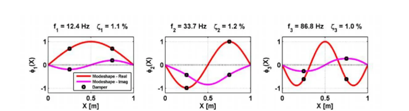
Figure 4: System with complex modes using negative damper

1

d

C

 at location

1 0.25

d

x  L and a

damper

2

d

C at location

2 0.75

d

x  L: Complex modeshapes for 50 Ns/m

d

C

  .

Figure 4 shows the first computed modes for the modified system of Figures 1(b) and 2, using

50 Ns/m

d

C





. Notice how, for this high level of modal complexity, the modal damping is kept

near the low value of the original system, showing the effectiveness of the proposed device.

5.2

Blind identification

Spectral results from the blind identification of the modal responses, obtained for the system with complex modes using first the real SOBI method and then the complex SOBI technique based on the analytic correlation matrix, are shown respectively in Figures 5 and 6. When the standard SOBI technique is applied to systems with complex modes, the modal extraction becomes imperfect so that residual modal peaks remain in all identified response spectra. The improvement stemming from the complex SOBI algorithm is unmistakable.

Figure 5. Case of complex modes (with 50 Ns/m

d

C

  ): Extracted modal auto-spectra using the standard (real) SOBI algorithm.

6 Conclusions

In this paper we explored several aspects of the blind identification of systems with strongly complex modes. Focus was on applicability of the SOBI technique for extracting the modal responses from analytic signals built from a set of vibratory responses using the Hilbert transform.

An interesting contribution of the present paper is a convenient computational procedure for directly obtaining the complex cross-correlation response matrix. Another contribution is the design of a convenient test system capable of displaying modes ranging from normal to highly complex, in a controlled manner, while keeping fairly constant low values of the modal damping.

Finally, based on numerical simulations of a physical multi-modal system subjected to distribute random excitation, we asserted the improved quality of the identified modal matrix and modal responses extracted using the complex SOBI technique based on analytic correlation matrices.

Acknowledgments

The authors acknowledge the financial support for this work, which was performed in the framework of a joint-research program co-funded by AREVA NP, EDF and CEA (France).

References

[1] James, G.H.; Carne, T.G.; Lauffer, J.P.; Nard, A.R. Modal testing using natural excitation.

Proceedings of the 10th International Modal Analysis Conference (IMAC1992), San Diego, USA, 3-7

February 1992.

[2] Brincker, R.; Ventura, C.E.Introduction to operational modal analysis. Wiley, Chichester (UK), 2015. [3] Rainieri, C.; Fabbrocino, G. (2014) Operational modal analysis of civil engineering structures: An

introduction and guide for applications. Springer, New York (USA), 2014.

[4] Belouchrani, A.; Karim, A.-M.; Cardoso, J.-F. A blind source separation technique using second-order statistics.IEEE Transactions on Signal Processing, Vol 45, 1997, pp 434-444.

[5] Poncelet, F.; Kerschen, G.; Golinval, J.-C.; Verhelst, D. Output-only modal analysis using blind source separation techniques. Mechanical Systems and Signal Processing, Vol 21, 2007, pp 2335-2358.

[6] Spina, D.; Valente, C.; Gabriele, S. Non classical modal parameters identification via dynamic response complexification.Proceedings of AIMETA-2009, Ancona, Italy, 14-17 September 2009. [7] McNeill, S.; Zimmerman, D. A framework for blind modal identification using joint approximate

diagonalization.Mechanical System and Signal Processing, Vol 22, 2008, pp 1526-1548.

[8] Caughey, T.; Okelly, M. Classical normal modes in damped linear dynamic systems. Journal of

Applied Mechanics, Vol 32, 1965, pp 583-588.

[9] Géradin, M.; Rixen, D.J. Mechanical vibrations: Theory and application to structural dynamics. Wiley, Chichester (UK), 2015.

[10] Feldman, M. Hilbert transform in vibration analysis. Mechanical Systems and Signal Processing, Vol 25, 2011, pp 735-802.

[11] McNeill, S. An analytic formulation for blind modal identification.Journal of Vibration and Control, Vol 18, 2011, pp 2111-2121.

[12] Tichavsky, P.; Yeredor, A. Fast approximate joint diagonalization incorporating weight matrices.IEEE