J. Braz. Soc. Mech. Sci. & Eng. vol.29 número4

Flávia Zinani

Member, ABCM fla@mecanica.ufrgs.br

Sérgio Frey

Emeritus Member, ABCM

frey@mecanica.ufrgs.br Federal University of Rio Grande do Sul - UFRGS Mechanical Engineering Department 90050-170 Porto Alegre, RS. Brazil

Galerkin Least-Squares Solutions for

Purely Viscous Flows of

Shear-Thinning Fluids and Regularized Yield

Stress Fluids

This paper aims to present Galerkin Least-Squares approximations for flows of Bingham plastic fluids. These fluids are modeled using the Generalized Newtonian Liquid (GNL) constitutive equation. Their viscoplastic behavior is predicted by the viscosity function, which employs the Papanastasiou’s regularization in order to predict a highly viscous behavior when the applied stress lies under the material’s yield stress. The mechanical modeling for this type of flow is based on the conservation equations of mass and momentum, coupled to the GNL constitutive equation for the extra-stress tensor. The finite element methodology concerned herein, the well-known Galerkin Least-Squares (GLS) method, overcomes the two greatest Galerkin shortcomings for mixed problems. There is no need to satisfy Babuška-Brezzi condition for velocity and pressure subspaces, and spurious numerical oscillations, due to the asymmetric nature of advective operator, are eliminated. Some numerical simulations are presented: first, the lid-driven cavity flow of shear-thinning and shear-thickening fluids, for the purpose of code validation; second, the flow of shear-thinning fluids with no yield stress limit, and finally, Bingham plastic creeping flows through 2:1 planar and axisymmetric expansions, for Bingham numbers between 0.2 and 133. The numerical results illustrate the arising of two distinct unyielded regions: one near the expansion corner and another along the flow centerline. For those regions, velocity and pressure fields are investigated for the various Bingham numbers tested.

Keywords: Bingham plastic, Carreau fluids, Yield Stress, Papanastasiou’s approximation, Galerkin Least-Squares

Introduction 1

This work is concerned with aspects of finite element simulation of isochoric flows of viscoplastic liquids, where the non-Newtonian constitutive law for the stress tensor is the Generalized Newtonian Liquid (GNL) model. Viscoplasticity is incorporated in this model by setting a yield stress, below which the material is assumed not to flow, into the viscosity function (see e.g. Bird et al. (1987) or Barnes (1999) for more details). Beyond the yield stress, most viscoplastic liquids are assumed to shear-thin, i.e., their viscosity decreases with the increase of strain rate. Viscoplastic materials are found in a wide range of applications associated with different industrial areas, such as: emulsions, polymer melts and solutions, food products, biological fluids, muds, asphalts, etc. Among the viscoplastic equations used in practice, the Bingham plastic is chosen in this paper for the numerical approximations. In order to achieve a computationally convenient formulation, (and also a more physically realistic behavior, see Souza Mendes and Dutra, 2004 and Roberts et al., 2001) a regularized version of the Bingham plastic constitutive model has been employed, following the approach proposed by Papanastasiou (1987).

The flows considered herein were approximated via a mixed finite element technique. The Galerkin Least-Squares method (GLS) (Hughes et al., 1986) is employed in order to avoid undesirable pathologies (spurious oscillations, locking) to which the classical Galerkin formulation would be susceptible. The Galerkin method in fluids suffers from two major difficulties. First, the need to satisfy the Babuška-Brezzi condition (Ciarlet, 1978) in order to achieve a compatible combination of velocity and pressure subspaces. Further, the inherent instability of central difference schemes in approximating advective dominated equations (Brooks and Hughes, 1982). The GLS method has the ability to circumvent Babuška-Brezzi condition and to generate stable approximations for highly

Paper accepted September, 2007. Technical Editor: Monica Feijo Naccache.

advective flows preserving good accuracy properties (Franca and Frey, 1992). This is achieved by adding residual-based terms to the classic Galerkin formulation, retaining its weighted residual structure and not damaging its consistency.

The numerical results section is divided in three sub-sections. The first is dedicated to the code validation. Newtonian and Non-Newtonian flows in a lid-driven cavity are investigated. The second deals about non-Newtonian flows of shear-thinning liquids through a planar contraction. In the third sub-section the simulations of flows of viscoplastic liquids are presented. These simulations comprise the numerical approximation of inertialess flows of Bingham fluids through sudden 2:1 planar and axisymmetric expansions. The stability of the numerical approximation is achieved for a wide range of Bingham numbers, which account for the fluid’s viscoplasticity. The flow dynamics is investigated through the visualization of pressure, velocity, viscosity and stress fields. It is important to emphasize that the numerical methodology adopted was able to capture well-defined unyielded regions at expansion corner and flow centerline. These regions are studied in detail throughout that section.

numerical and experimental comparisons. Reis Junior and Naccache (2003) simulated viscoplastic flows through contractions via a finite volume method, with the plasticity behavior modeled by the Carreau equation subjected to a very high low-shear-rate-viscosity. Neofytou and Drikakis (2003) investigated the flows of three different fluid models (Casson, Quemada and power-law) in a sudden expansion channel. Zinani and Frey (2006) employed a GLS method to approximate the flow of Casson fluids through a planar expansion. They examined the relation between vortex formation and flow plasticization in the corner downstream the expansion, emphasizing that highly viscoplastic liquids tend to inhibit vortex formation. Recently, Mitsoulis and Huilgol (2004) simulated entry flows of Bingham plastics in expansions by a finite element method, computing the vortex size and intensity, as well as the entrance correction, as functions of the material yield stress. Their results are employed as a base of comparison for our results.

Nomenclature

a incremental vector B GLS functional Bn Bingham number

C0 space of continuous functions Cu Carreau number

Ch finite element partition D strain rate tensor div divergence operator F GLS functional F momentum load vector f vector of body forces G incompressibility matrix grad gradient operator

H1 Sobolev functional space hK element size

I identity tensor

ID, IID, IIID invariants of the strain rate tensor

int(i) value of i truncated to an integer J Jacobian matrix

K element domain K momentum diffusive matrix L2 Hilbert functional space L Characteristic length

m Papanastasiou’s approximation parameter N momentum advective matrix

n outward normal unit vector n power-law exponent P pressure functional space p pressure field q pressure variation function r position vector

R residual vector

ℜ set of real numbers Re Reynolds number

Rk polynomial functional space of degree k T stress tensor

t stress vector

t time

U vector of degrees of freedom u admissible velocity field

ui velocity component in the i direction u0 characteristic velocity

V velocity functional space v virtual velocity field W vorticity tensor

Greek Symbols

γ

& magnitude of tensor D Γ domain boundary η viscosity function

λ time parameter in Carreau model η0 zero-shear-rate viscosity η∞ infinite-shear-rate viscosity ηc characteristic viscosity ηp plastic viscosity µ Newtonian viscosity ν kinematic viscosity ρ mass density

τ magnitude of stress, GLS stability parameter τ0 yield stress

Ω problem domain ξ upwind function Subscripts

a advection field

g Dirichlet boundary condition

h finite element approximation, Neumann boundary condition

K finite element τ GLS stabilized matrix Superscripts

nsd number of space dimensions *

dimensionless

Mechanical Modeling

The problems studied herein are defined in an open bounded domain Ω ⊂ ℜ2 with polygonal boundary Γ such that,

,

, 0

g h

g h g

Γ = Γ Γ

 

Γ Γ = ∅ Γ ≠

 U I

(1)

where Γg is the portion of Γ over which the Dirichlet boundary conditions are imposed and Γh the portion of Γ where the Neumann boundary conditions are prescribed.

The Continuity Equation

The mass of a mechanical body is invariant with time. Mathematically, this conservative principle may be expressed by

0

d d

dt_Ω

∫

ρ

Ω = (2)

where ρ is the mass density. Applying the Reynolds transport theorem (Truesdell and Toupin, 1960) to Eq. (2), the differential form of the mass conservation equation may be achieved (Gurtin, 1981),

div( ) 0

t

ρ

ρ

∂

+ =

∂ v (3)

The Motion Equation

In fluid motion, all dynamic interactions may be described in terms of the forces acting on the fluid, which are described by balance laws that are valid for any arbitrary continuous portion of the fluid. Classically, three distinct types of forces are considered in Mechanics: internal contact forces, surface forces and body forces. All of them are related to the fluid motion through Euler dynamical axioms (Truesdell and Toupin, 1960).

Principle of Momentum Balance: The rate of change of momentum in a fluid volume Ω is equal to the total force acting on it.

( )

d

d d d

dt

∫

Ω

ρ

v Ω =

∫

Ωf Ω +

∫

Γt n Γ (4)

Principle of Angular Momentum Balance: The rate of change of angular momentum in a fluid volume Ω is equal to the sum of the moments acting on it.

( )

d

d d d

dt

∫

Ωr×

ρ

v Ω =

∫

Ωr f× Ω +

∫

Γr t n× Γ (5) where r denotes the position vector.

In order to establish the fluid motion equation, Cauchy theorem is enunciated (Gurtin, 1981), which has, as main assertion, the linearity of the stress vector t(n): Let (t,n) be a system of forces of a body in motion. The necessary and sufficient condition so that the laws of momentum conservation are satisfied is the existence of a symmetrical tensor field T – Cauchy tensor – such as: t(n)=Tn, satisfying the motion equation:

div

ρ

v&= T f+ (6)

Material Behavior

Although Cauchy Theorem describes the form of the contact forces, stated for any continuous body, the way in which materials deform under arbitrary dynamic conditions is not stated by this theorem. In addition, the behavior of continuous bodies differs drastically with respect to the relation between internal contact forces (accounted by the stress tensor, T) and their motion and deformation. This relation is described mathematically by the so-called rheological or material constitutive equations. The constitutive equations are constructed in order to obey certain rules that assure their physical meaning and generality. These rules are summarized in some principles, according to Astarita and Marrucci (1974) and Slattery (1999): the principle of determinism, principle of local action, principle of frame indifference, principle of fading memory and the satisfaction of the second law of thermodynamics.

Being so, the dependence of T upon the body motion and deformation might give a function of the type,

(

, grad

)

=

T T v v (7)

Decomposing the tensor gradv in symmetric and skew-symmetric parts, that is gradv=D+W, one has that the symmetric tensor D - called the strain rate tensor – is a frame indifferent tensor while the skew-symmetric tensor W – called the vorticity tensor - is not. In addition the velocity field v is not a frame indifferent field. Therefore, a constitutive equation for T written only in terms of D is also a frame indifferent function (Gurtin, 1981).

The relation between T and D that obeys the principles above is based on the representation theorem for isotropic linear tensor functions (Gurtin, 1981) (4):

2

1 2 3

( )=ψ (ID,IID,IIID) +ψ (ID,IID,IIID) +ψ (ID,IID,IIID)

T D I D D (8)

where ID, IID and IIID are the invariants of D. When the fluid is at

rest (D=0), it develops a uniform field of hydrostatic stress, which is identified as the hydrodynamic pressure, p. In this case,

p

= −

T I (9)

The generalized Newtonian liquid (GNL) is a model based on Eqs. (8) and (9), by neglecting the quadratic term in Eq. (8) and considering the phenomena that occur in viscometric flows. Many flows of industrial interest are nearly viscometric. In this type of flow, the invariants ID and IIID are null (Gurtin, 1981), and the most

relevant material function is the viscosity, which is represented by the coefficient of the second term on the right side of Eq. (8). The GNL model incorporates the viscosity dependence on strain rate, which is commonly observed in many polymeric fluids. This model is mathematically written as:

2 ( )

p

η γ

= − +

T I & D (10)

where η(

γ

&) is the viscosity function. The scalar

γ

& is defined as the magnitude of the strain rate tensor (Slattery, 1999), which corresponds to the strain rate in viscometric flows:

1 2 2 1 2

(2II ) (2tr )

γ

&= D = D (11)

In the case where the viscosity is assumed constant, Eq. (10) reduces to the classical Newtonian model, with η=µ.

Despite the GNL model does not predict normal stress differences in shear motions, it is useful in modeling a large scope of fluids in isochoric motion and shear dominated flows, when the most important phenomena are those caused by changes of viscosity. The flexibility of a strain rate dependent viscosity function allows the prediction of some commonly observed effects in shearing flows, as shear-thinning, also called pseudoplasticity (viscosity decrease with the increase of strain rate), shear-thickening (viscosity increase with the increase of strain rate), and also viscoplasticity (the fluid does not deform if the applied stress lies under a yield stress, and beyond the yield stress the fluid presents shear-thinning).

A widespread empirical model for the viscosity function η(

γ

&) is the four-parameter Carreau fluid (Bird et al., 1987), which is employed to model shear-thinning fluids. It is written as:

1 2 ₂ 0

( ) ( ) 1 ( )

n

η γ

η

η

η

λγ

−

∞ ∞  

= + − _ + _

& & (12)

where η0 is the zero shear-rate viscosity,η∞ the infinite shear-rate

viscosity, n represents the power-law exponent and λ a time constant. The Carreau dimensionless number, Cu, is given as:

0

Cu L

u

λ

= (13)

1

( ) _K n

η γ

_{& =}

γ

_&−

(14)

with K the consistency index, which is equivalent to η0λn-1 for the Carreau model when λ tends to infinity.

The viscoplastic equation for the stress-strain behavior of a Bingham plastic was proposed in the following form for viscometric flows (Bird et al., 1987):

0 0

0

for 0 for

p

τ

τ

η γ

τ

τ

γ

τ

τ

= + >

= ≤

&

& (15)

where τ is the shear stress and

γ

& the strain rate. The symbol ηp stands for the plastic viscosity. For general flows, τ is assumed as the magnitude of the extra-stress tensor, ττττ=T+pI, given by

(

₂

)

1 2

1 2 tr

τ

= τ (16)

and

γ

& is defined as in Eq. (11). The viscosity function is then given as:

0

0

( )

τ

_p for

η γ

η

τ

τ

γ

= + >

&

& (17)

For

τ

≤

τ

₀, the viscosity function goes to infinity as τ approaches zero. Papanastasiou (1987) proposed a modification in the Bingham plastic equation by introducing the material parameter m, which replaces the discontinuity of the viscosity function by an exponential stress growth for low strain rates. In this way, the equation is valid for both yielded and unyielded zones. Papanastasiou’s modification gives rise to the following continuous viscosity function:

(

)

0 _{1 exp}

p m

τ

η η

γ

γ

= + _ − − & _

& (18)

The Bingham dimensionless number is defined as follows

0 0 Bn p L u

τ

η

= (19)

The viscosity of a fluid is employed in order to define a flow’s Reynolds number, along with other flow parameters (velocity, mass density and length). In the case of GNL, a characteristic fluid’s viscosity, ηc, must be set in order to define a Reynolds number. In this paper, the characteristic viscosity for the Carreau fluids is taken as the zero shear rate viscosity, η0; for the Bingham fluids the plastic viscosity, ηp; and for Newtonian fluids the Newtonian viscosity µ. So, The Reynolds number is defined as:

0 Re c u L

ρ

η

= (20)

Finite Element Methodology

The equations of continuity and momentum conservation (Eq. (3) and Eq. (6) respectively), plus the GNL constitutive equation (Eq.(10)) in a domain Ω⊂ℜ2

are used to construct the following boundary-value problem:

[

]

( )

( )

grad 2 div grad in

div 0 in

on

2 ( ) on

g g

h h

p

p

ρ

η γ

ρ

η γ

− + = Ω

= Ω

= Γ

− + = Γ

 

 

u u D f

u

u u

I D u n t

&

&

(21)

where u is the admissible velocity field, p the pressure field,

η γ

( )

& the viscosity function (Eq. (18)), D the strain rate tensor, n the unit outward vector and f the vector of body forces.

The system defined by Eqs. (21) was approximated by a finite element method using a stabilization scheme which was based on Galerkin Least-Squares formulations developed in (Hughes et al., 1986, Franca and Frey, 1992, and references therein). Over the domain Ω a finite element partitionC_h, consisting of convex quadrilateral Q1 elements in ℜ2

was performed in the usual way (Ciarlet, 1978),

1 2 , 1, 2

h

K K C

K K K K Ch

∈

Ω= Ω

 

Ω Ω = ∅ ∀ ∈

 U I

(22)

Throughout the article, the functional spaces L2( )Ω , 2

0( )

L Ω ,H1( )Ω andH1₀( )Ω are defined in the usual way,

{

}

{

}

{

}

2 2 2 2 0

1 2 2

1 2 2

0

( ) { | } ( ) ( ) | =0

( ) ( ) | ( )}, 1,

( ) ( ) | ( ) | 0 on , 1,...,

i

i g

L q q d

L q L qd

H v L v x L i nsd

H v L v x L v i nsd

Ω

Ω

Ω = Ω < ∞

Ω = ∈ Ω Ω

Ω = ∈ Ω ∂ ∂ ∈ Ω =

Ω = ∈ Ω ∂ ∂ ∈ Ω = Γ =

∫

∫

(23)

Besides,

( )

⋅ ⋅, and 0

⋅ represents, respectively, the L2 _inner product and the norm on Ω, and

_{( )}

⋅ ⋅, _K and

0,K

⋅ the L2 inner product and the norm on the element domain Κ, respectively.

The Galerkin Least-Squares Formulation

In order to approximate the velocity and pressure, the following spaces of approximation functions are employed, which are usual in fluid dynamics (Ciarlet, 1978):

1 0

{ ( )nsd ( )nsd, }

h = ∈H Ω K∈R Kk K∈Ch

V v v (24)

1

{ ( ) ( ) , , on }

g nsd nsd

h = ∈H Ω K∈R Kk K∈Ch = g Γg

V v v v u (25)

0 2

0

{ ( ) ( ) ( ), }

h K l h

P = p∈C Ω IL Ω p ∈R K K∈C (26)

where Rk and Rl denote the polynomial spaces of degrees k and l, respectively.

Based on the finite element subspaces defined by Eq. (24)-(26), a Galerkin Least-Squares formulation may be introduced to approximate system (21) as: find the pair (uh, ph) ∈Vhg x Ph such as:

(

_h, _h; ,

)

(

,

)

(

_{h h}

)

B u p vq =F vq ∀ V ×P (27)

(

)

(

[

]

)

(

( )

)

(

) (

)

[

]

( )

(

)

(

[

]

( )

)

(

)

, ; , grad , 2 ( ), ( ) div , div ,

grad 2div( )) grad , Re grad 2div( )) grad

h

K _K

K C

B p q p q

p q

ρ η γ

ρ η γ τ ρ η γ

∈

= + − − +

+

∑

− + − −

u v u u v D u D v v u

u u D(u v u D(u

&

& & (28)

and

(

,

) (

,

) (

,

)

(

,

(

Re

)

(

[

grad 2div(

]

( )

( )) grad

)

)

h h

h K _K

K C

F q

ρ

_Γ

ρ τ

ρ

η γ

q

∈

= + +

∑

− −

v f v t v f v u & D v (29)

with the terms within the sums of Eq. (28)-(29) evaluated elementwise and its stability parameter τ being the same as in Franca and Frey (1992), for the linear Newtonian fluid

(Re ) (Re ), with Re

2 4 ( )

k p K

K

K K K

p

m h

h

τ ξ

η γ ρ

= = u

u & (30)

Re , 0 Re 1 (Re )

1, Re 1

K K

K

K

ξ = ≤ <

≥

 (31)

1 min , 2

3

k k

m = _ C _

  (32)

1 1 1, , 1 max , p nsd p j j p j j nsd u p u p = =  

_{  ≤ < ∞}



= 

 _{= ∞}



∑

u (33)

2 2

2

0, 0

div ( ) ( )

h

k K K h

K C

C h

∈

≤ ∈

∑

D v D v v V (34)

Remark 1: For the sake of analysis, a linear version of the formulation of Eqs. (27)-(34) must be introduced. Based on Oseen’s improvement for the Stokes solution (Landau and Lifchitz, 1971). This set of equations reduces to the following, subjected to appropriated boundary conditions,

(grad ) grad 2 div ( ) 0 in

div 0 in

p

ρ

+ −

η

−

ρ

= Ω

Ω

a

u v D u f

u = (35)

where va is a given advection field and η assumed constant

throughout the domain, linearizing the problem. Setting the stabilization parameter τto zero, the stabilized formulation defined by Eq.(27)-(34) reduces to the classical Galerkin approximation for this version of system of Eq.(21). The instability of Galerkin approximation (35) for advective dominated flows is due to the lack

of coercivity of its bilinear form. Choosing (u, p)=(v, −q) and selecting v∈H1₀( )Ω nsd, it follows that

2 0

( , ; , ) 2 ( ) ( , ) _{h h}

B v −q v q ≥

ν

D v ∀ v q ∈V ×P (36)

Therefore, when the kinematic viscosity ν=µ/ρ tends to zero, the linear Galerkin approximation will be polluted by spurious oscillations, generating physically unreal solutions.

Applying the analysis introduced in Franca and Frey (1992) to this context, but with a non-null stability parameter τ defined as in Eq. (30)-(34), the stability features of the GLS method follow immediately. The stability lemma runs as follows:

(

)

(

2 1 2

)

0

1

( , ; , ) 2 ( ) (grad ) (grad ) ( , )

2 h h

Bv−qvq ≥ ν D v +τ v va+ p ∀vq∈V×P

(37)

Matrix Problem

Discretization of Eq.(27)-(34) is carried out by expanding the trial functions u, p, and v, q in terms of their finite element basis or shape functions. This leads to a set of semi-discrete equations, which, in the residual form is written as:

( )=

R U 0 (38)

where U is the vector of degrees of freedom of uh

and ph, and R(U) is given by the set of matrices

In Eq. (39), matrices [K] and [G] are, respectively, originated by the diffusive and pressure terms of Eq.(27)-(29), and N(u), GT, F by the advective, incompressibility and body force ones. (The N(u)τ,

[K]τ, [G]τ, N(u)τ, and Fτ in Eq. (39) are generated by the

Least-Squares terms of Eq.(27)-(34).) To solve system defined by Eq.(38)-(39), a quasi-Newton method (Dalquist and Bjorck (1969)) has been implemented, with convergence criteria of maximum residual norm equal to 10-6. As initial solution estimates, null velocity and pressure fields were employed. The Jacobian matrix for this method is given below (Eq. (40)), and solution algorithm is the same as the one elucidated in Zinani and Frey, 2006.

* * * * * * * * * *

( ) ( ) ( ( ), ) [ ( ( )) ( ( ), )] [ ( ( ), )] T ( ( ), )

τ

η γ

η γ

τ

η γ

τ

η γ

τ

η γ

= + + + + + + − −

R U N u u N & u u K & K & u u G G & u p G u F F & u ₍₃₉₎

( ( ), ) ( ( ), )

( )

( ) ( ) ( ( ), ) ( ( )) ( ( ), )

( ( ), ) ( ( ), )

( ( ), ) T

τ τ

τ τ

τ τ

τ

η γ η γ

η γ η γ η γ

η γ η γ

η γ ∂ ∂ ∂ = + + + + + + + ∂ ∂ ∂ ∂ ∂ + + + + − ∂ ∂

N u K u

N u

J U N u u N u u K K u u

u u u

G u F u

G p G u G

u u

& &

& & &

& &

&

Numerical Results

The GLS formulation defined by Eq.(27)-(34) was employed in order to approximate GNL flows. All computations have used a non-linear finite element code for fluids under development at the Laboratory of Computational and Applied Fluid Mechanics (LAMAC), Mechanical Engineering Department, UFRGS.

Flows in a Lid-Driven Cavity

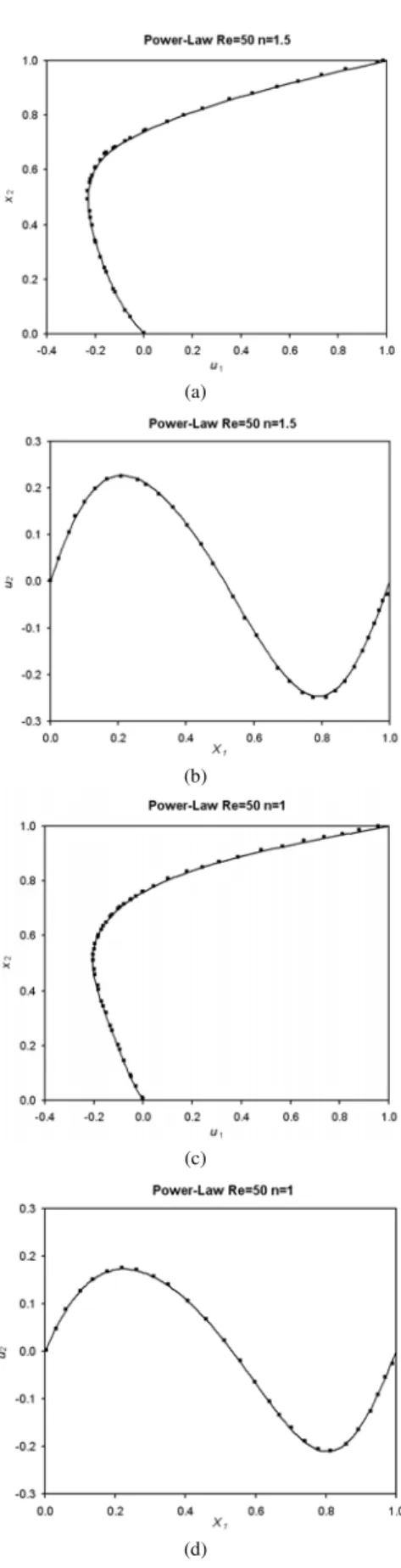
As a check for the computational implementation of the GLS formulation defined by Eq.(27), the approximation of non-Newtonian flows subjected to mild advective transport of momentum was implemented. The lid-driven cavity problem was built in the usual manner (Fig. 1), with square cavity geometry of length L. The velocity boundary conditions were impermeability and non-slip at cavity walls except the upper one, on which a horizontal velocity u0 was prescribed. The power-law viscosity model was employed in order to allow the comparison with previous work (Neofytou, 2005). In the Reynolds number definition (Eq. (20)), the characteristic viscosity employed was ηc=K(u0/L)(n−1). A Reynolds number equal to 50 was investigated using three values of the power-law index, n: n=1.5, n=0.5 and n=1. A 120x120 Q1/Q1 finite element mesh was used. The Newtonian version of this problem is exploited in Zinani and Frey, 2006.

Figure 1. Problem statement for the lid-driven cavity.

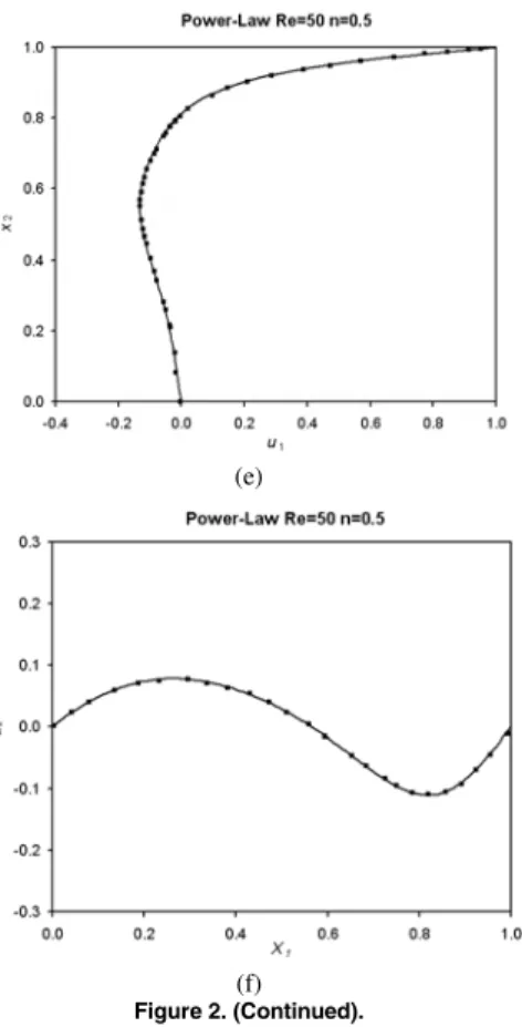
In Fig. 2 the results for the horizontal velocity in the line x1=0.5L and the vertical velocity in the line x2=0.5L are shown. The dots correspond to the results of Neofytou (2005), and our results are represented by filled lines. The results of the present paper agree well with the literature. One may observe that, in relation to the Newtonian fluid (n=1), the shear-thinning fluid (n=0.5) reduces drastically the velocity gradients, while the dilatant fluid (n=1.5) increases them.

(a)

(b)

(c)

(d)

(e)

(f)

Figure 2. (Continued).

Shear-Thinning Flow Through a Sudden Contraction In this section, the Carreau fluid flow trough a planar 4:1 sudden contraction is studied. The problem statement is given in Fig. 3. Considering the symmetry, half problem’s actual domain is employed to build the geometric model. The boundary conditions for this problem are: fully developed Newtonian velocity profile with mean velocity u0/4 in the inlet, non-slip and impermeability at walls (ui=0, i=1,2), symmetry in x2=0 (u2=0, ∂u₁ ∂x₂=0), and free traction at the outflow boundary. The parameters L and u0 are used to calculate each case’s Reynolds number (Eq. (20)), along with the characteristic viscosity of the Carreau model, η0. In the Carreau viscosity function, the infinite shear-rate viscosity, η∞, was taken equal to zero, so that three dimensionless parameters are needed to define the flow: Re, Cu and n.

2L

L/2

u

0

x

1

x

2

Figure 3. Problem statement for the Carreau flow through a sudden 4:1 contraction.

This analysis is based in two Reynolds number values for a Newtonian fluid, Re=1 and Re=100, and two Carreau numbers (Eq. (13)) and n index values for the non-Newtonian fluids (for Re=1): Cu=0.5 and Cu=50, and n=0.1 and n=0.5. The effects of the fluid’s shear-thinning in the flow dynamics are investigated, i.e. how the local viscosity decrease in the high shear rate regions affects the

flow. A mesh dependency analysis was performed with three meshes, comprised of 3120 (m1), 5362 (m2) and 7154 (m3) elements. The results were started to be mesh independent from mesh m2.

The GLS formulation produced stable numerical results for Newtonian flows, for Reynolds numbers between 0 and 100, and also for the non-Newtonian flows corresponding to the values cited above for the Carreau model.

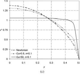
In Fig. 4, the horizontal velocity profiles for the Newtonian and shear-thinning fluids are depicted, for Re=1: (a) upstream the contraction, representing a fully developed profiles, not disturbed by the contraction; (b) at a distance L upstream the contraction plane, (c) at the contraction plane. In these graphics, y=x2/L and u*=u1/u0, the dimensionless horizontal velocity. In the fully-developed profile (a), the typical flattened profile is observed in the profile of the higher Carreau number fluid (Cu=50). The low Carreau number fluid (Cu=0.5) has the same velocity profile as the Newtonian fluid, which means that the viscosity of this fluid does not decrease, i.e., it is kept in the viscosity plateau of this model, where viscosity is constant and the fluid presents a near Newtonian behavior, for very low strain rates. The same occurs with the profile just upstream the contraction plane (b): the low Cu and the Newtonian fluids present identical velocity profiles, while the high Cu fluid presents a much more flattened profile, but with the same tendency of acceleration in the symmetry line. In the contraction plane (c), the fluid experiments much deformation and even the low Cu fluid presents a different profile from the Newtonian one. The high Cu fluid presents a flattened profile, due to the high deformation region that is formed because of the contraction.

(a)

(b)

(c)

Figure 4. (Continued).

Figure 5 shows graphics of the pressure drop along the symmetry plane for the Newtonian fluid with Re=1 and Re=100, and the Carreau fluids with Re=1 and various fluid’s parameters. In part (a) the pressure drops obtained for the Newtonian fluid at Re=1 and the shear-thinning fluids with low Cu are compared. One may observe that the pressure levels are of the same magnitude, despite shear-thinning reduces the total pressure drop. In part (b) the pressure drops for the high Cu fluids are shown. One may observe that the levels of pressure fall much lower than the Newtonian fluid flowing with Re=1, and that they fall in the same range of magnitude than a Newtonian fluid flowing with Re=100. This phenomenon is a consequence of the viscosity reduction due to shear-thinning, which may reduce the resistance to flow in orders of magnitude, as in this example. Another interesting feature is that the slope of the shear-thinning curves differ much from the Newtonian in the region downstream the contraction, i.e., where deformation by shear is more severe and shear-thinning is more pronounced.

(a)

Figure 5. Pressure drop along the symmetry plane: (a) Newtonian with Re=1 and low Cu fluids, (b) Newtonian with Re=100 and high Cu fluids with Re=1.

(b)

Figure 5. (Continued).

Bingham Flow Through 2:1 Expansions

In this section, inertialess flows of regularized Bingham fluids (Eq. (18)) through 2:1 sudden expansions are studied (as illustrated in Fig. 6), employing both planar and axisymmetric coordinate systems. The geometry total length is of 60L, to guarantee the inflow development upstream and downstream the expansion. The boundary conditions were: fully developed Newtonian velocity profile with mean velocity u0 in the inlet, non-slip and impermeability at walls (ui=0, i=1,2), symmetry in x2=0 (u2=0,

1 2 0

u x

∂ ∂ = ), and free traction at the outflow boundary. The values of L, u0, and the viscosity ηc have been set equal to unity. A detail of the finite element mesh is seen in Fig. 7. The results were obtained for Bingham numbers (Eq.(19)) from Bn=0 (Newtonian fluid) to Bn=133, employing a finite element mesh with 10,640 Q1/Q1 elements. The parameter m in Eq. (18) was taken as great as to give mL/u0=1000, as suggested in Mitsoulis and Zisis (2001) in order to reproduce the Bingham model.

2L L

u

0

x₂

x

1

Figure 6. Flow in a 2:1 expansion, problem statement.

Figure 7. A detail of the employed finite element mesh.

black zones in the figure), which are located near expansion corner and around flow centerline. While stagnant velocities at the corner originate the former (stagnant) region, the latter one is due to the growth of a plug flow at the centerline (rigid body motion). These regions tend to grow as the Bingham number increases, for the yield limit gets higher. It is also possible to observe that the unyielded zones are greater in the planar cases, since the flow is only subjected to the shear stresses in the upper and lower walls, while in the axisymmetric cases the whole flow region is surrounded by the walls, which shear the fluid yielding the flow.

(a)

(b)

(c)

(d)

Figure 8. Planar geometry. Unyielded zones for (a) Bn=0.2; (b) Bn=3.9; (c) Bn=27.1; (d) Bn=127.

(a)

(b)

(c)

Figure 9. Axisymmetric geometry. Unyielded zones for (a) Bn=0.2; (b) Bn=4.76; (c) Bn=11.29; (d) Bn=133.

(d)

Figure 9. (Continued).

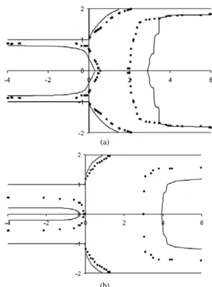
The flow of Bingham plastics in expansions has been studied by Mitsoulis and Huilgol (2004). For the specific case of flows trough a planar expansion, these authors present results for the yield surfaces, i.e., the limiting surfaces between yielded and unyielded zones. Fig. 10 depicts the superposition of the yield surface position obtained using the GLS formulation of Eq. (27)-(34) (lines) and the results of Mitsoulis and Huilgol (2004) (dots), for two Bingham numbers, Bn=127, planar flow and Bn=11.29, axisymmetric flow. It is possible to see that the GLS results agree well with those of Mitsoulis and Huilgol (2004). In the planar case, the results present yielded zones with the same width but distinct lengths. In the axisymmetric case, the width of the present results seem also smaller that that of Mitsoulis and Huilgol (2004).

(a)

(b)

Figure 10. Yield surfaces, comparison of GLS results (lines) with Mitsoulis and Huilgol, 2004 (dots). (a) Planar Bn=127, (b) axisymmetric, Bn=11.29.

(a)

(b)

(c)

(d)

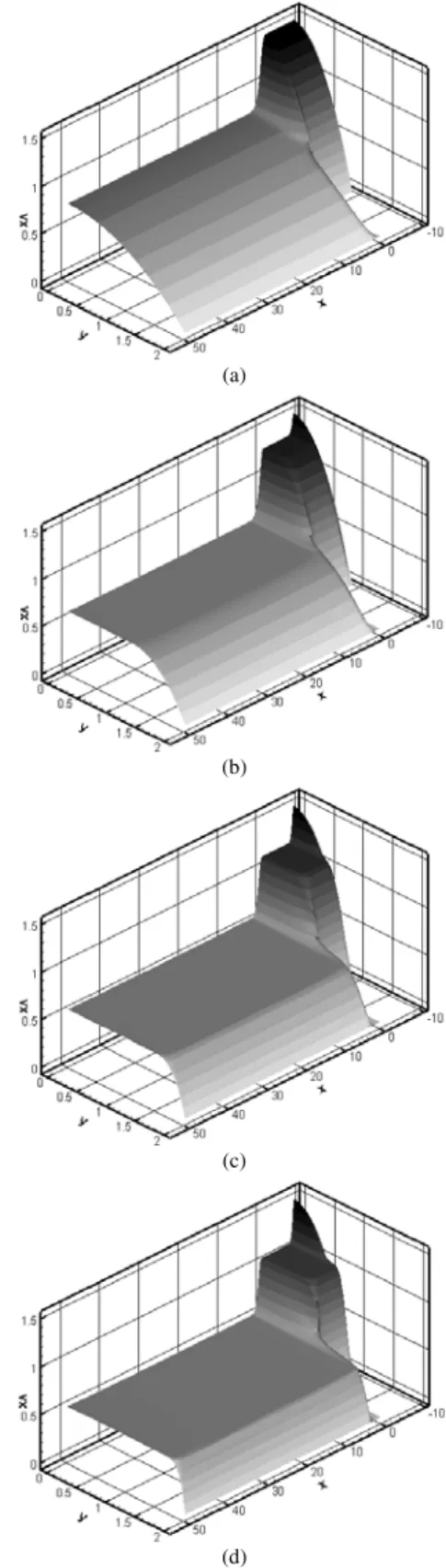
Figure 11. Horizontal velocity elevation plot for planar flows: (a) Bn=0.2; (b) Bn=2, (c) Bn=10, (d) Bn=110.

(a)

(b)

(c)

(d)

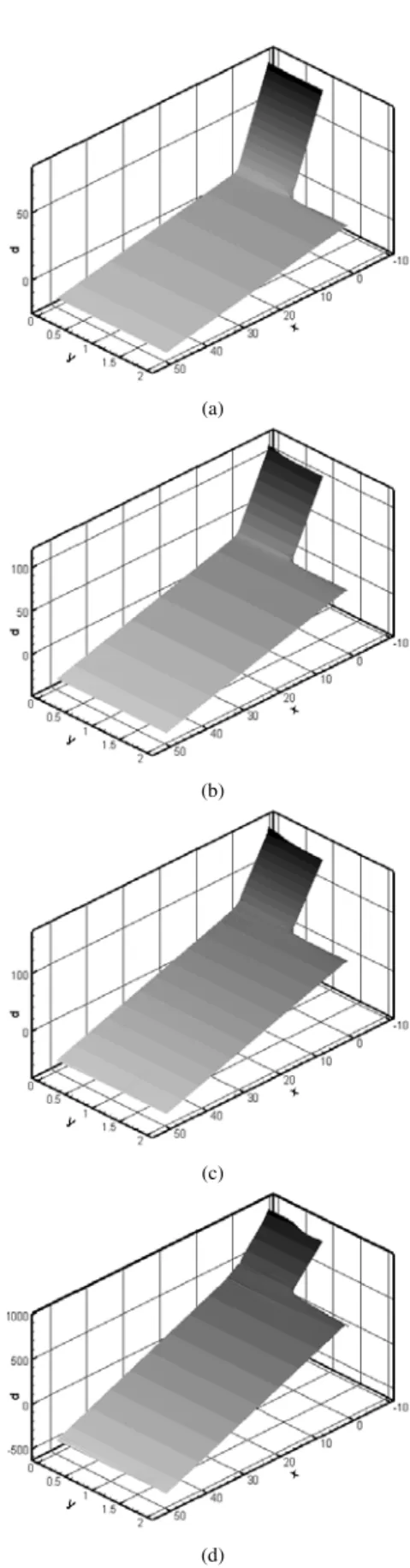
Figures 13 and 14 illustrate the pressure drops throughout the planar channel. One observes that the higher the Bn, the higher the pressure drop. This feature may be explained by the high drag caused by the unyielded zones. The perturbation in the pressure field caused by the imposition of boundary conditions may be noticed, but it is also noticed that they do not disturb that field in the region of interest, i.e., near the expansion.

(a)

(b)

(c)

(d)

Figure 13. Pressure contours and elevation for planar flows: (a) Bn=0.2; (b) Bn=3.9, (c) Bn=27.1, (d) Bn=127.

(a)

(b)

(c)

(d)

Conclusions

This work exploited the features of a Galerkin Least-Squares finite element method in the approximation of purely viscous non-Newtonian flows. The method was efficient in stabilizing both pressure and velocity fields, circumventing the compatibility conditions between their subspaces. The method was also capable to stabilize the advective dominated zones that have arisen due to shear-thinning, to keep the regions of high viscosity gradients stable, and also to be implemented in an axisymmetric coordinate system. Such features were demonstrated in the approximation of Carreau and Bingham fluids. In the case of flow of Carreau fluids through a contraction, the effects of shear-thinning were the flattening of the velocity profile in the contraction plane and the reduction of pressure drop due to viscosity reduction. In the cases of flows of Papanastasiou regularized Bingham fluid through expansions, the effect of increasing the yield limit (by increasing its dimensionless counterpart, the Bingham number) was to increase considerably the pressure drop due to the formation of a growing yielded zone in the contraction plane. In addition, the flattening of the velocity profile was also noticed.

Acknowledgments

F. Zinani and S. Frey thank the support provided by MCT/CNPq for the grants no. 154619/2006-0 and no. 50747/1993-8, respectively, and also the financial support provided by project no. 472094/2006-8. F. Zinani also acknowledges the agency CAPES for the doctoral grant 2002-2006.

References

Astarita, G., Marrucci, G., 1974. “Principles of non-Newtonian fluid mechanics”. McGraw-Hill, Great Britain.

Abdali, S.S., Mitsoulis, E., Markatos, N.C., 1992, “Entry and Exit Flows

of Bingham Fluids”, Journal of Rheology, Vol. 36, pp. 389-407.

Barnes, H.A., 1999, “The Yield Stress – a Review or ‘παντα ρει’ –

Everything Flows?”, Journal of Non-Newtonian Fluid Mechanics, Vol. 81,

pp. 133-178.

Bird, R.B., Armstrong, R.C., Hassager, O., 1987, “Dynamics of polymeric liquids”, Vol. 1, John Wiley and Sons, USA.

Brooks, A.N., Hughes, T.J.R., 1982, “Streamline Upwind/Petrov-Galerkin formulations for convective dominated flows with particular

emphasis on the incompressible Navier-Stokes equations”, Comp. Meths.

Appl. Mech. Eng., Vol. 32, pp. 199-259.

Ciarlet, P.G., 1978, “The Finite Element Method for Elliptic Problems”, North-Holland, Amsterdam, pp. 530.

Dahlquist, G., Bjorck, A., 1969, “Numerical Methods”, Prentice-Hall, Englewood Cliffs.

Franca, L.P., Frey, S., 1992, “Stabilized finite element methods: II. The

incompressible Navier-Stokes equations”, Comp. Meths. Appl. Mech. Eng.,

Vol. 99, pp. 209-233.

Franca, L. P., Frey, S., Hughes, T. J. R., 1992. “Stabilized finite element

methods: I. Application to the advective-diffusive model”. Computer

Methods in Applied Mechanics and Engineering., Vol. 95, pp. 253-276. Ghia, U., Ghia, K. N., Shin, C. T., 1982. “Hi-Re solution for incompressible flow using the Navier-Stokes equationsand the multigrid

method”. J. Comput Physics. Vol. 48, pp. 387-411.

Gurtin, M.E., 1981, “An Introduction to Continuum Mechanics”, Academic Press, NY, USA.

Hammad, K. J., Ötügen, M.V., Vradis, G.C., 1999, “Laminar flow of a nonlinear viscoplastic fluid through an axisymmetric sudden expansion”,

Journal of Fluids Engineering, Vol. 121, pp. 488-495.

Hannani, S.K., Stanislas, M., Dupont, P., 1995, “Incompressible Navier-Stokes computations with SUPG and GLS formulations – a comparison

study”, Computer Methods in Applied Mechanics and Engineering, Vol. 124,

pp. 153-170.

Hughes, T.J.R., Franca, L.P., Balestra, M., 1986, “A new finite element formulation for computational fluid dynamics: V. Circumventing the Babuška-Brezzi condition: a stable Petrov-Galerkin formulation of the

Stokes problem accommodating equal-order interpolations”. Comp. Meths.

Appl. Mech. Eng., Vol. 59, pp. 85-99.

Jay, P., Magnin, A., Piau, J.M., 2001, “Viscoplastic Fluid Flow Through

a Sudden Axisymmetric Expansion”, AIChE Journal, Vol. 47, pp.

2155-2166.

Landau, L., Lifchitz, E., 1971. “Mécanique des Fluides”. Edições Mir, Moscou.

Mitsoulis, E., Huilgol, R.R, 2004, “Entry flows of Bingham plastics in

expansions”, J. Non-Newtonian Fluid Mech., Vol. 122, pp. 45-54.

Mitsoulis, E., Zisis, T., 2001, “Flow of Bingham plastics in a lid-driven

square cavity”, J. Non-Newtonian Fluid Mech., Vol. 101, pp. 173-180.

Neofytou, P., Drikakis, D., 2003, “Non-Newtonian flow instability in a

channel with a sudden expansion”, Journal of Non-Newtonian Fluid

Mechanics, Vol. 111, pp. 127-150.

Pak, B., Cho, Y.I., Choi, S.U.S., 1990, “Separation and reattachment of

non-Newtonian fluid flows in a sudden expansion pipe”, Journal of

Non-Newtonian Fluid Mechanics, Vol. 37, pp. 175-199.

Papanastasiou, T.C., 1987, “Flows of materials with yield”, J. of

Rheology, Vol. 31, pp. 385-404.

Pham, T.V., Mitsoulis, E., 1994, “Entry and exit flows of Casson

fluids”, The Canadian Journal of Chemical Engineering, Vol. 72,

pp.1080-1084.

Reis Junior, L.A., Naccache, M.F., 2003, “Analysis of non-Newtonian flows through contractions and expansions”, Proceedings of the XVII COBEM International Congress of Mechanical Engineering, São Paulo.

Roberts, G. P., Barnes H. A., Carew, P., 2001, “Modelling the flow

behaviour of very shear-thinning liquids”, Chemical Engineering Science,

Vol. 56, pp. 5617-5623.

Slattery, J.C., 1999. “Advanced Transport Phenomena”. Cambridge University Press, U.S.A.

Souza Mendes, P. R., Dutra, E., 2004, “Viscosity function for yield stress liquids”, Applied Rheology, Vol. 14, pp. 296-302.

Truesdell, C., Toupin, R.A., 1960, “The classical field theories”, In: S. Flugge, Handbuch Der Physic, Vol. 3/1, Springer-Verlag, Berlin.

Vradis, G.C., Ötügen, M.V., 1997, “The axisymmetric sudden expansion

of a non-Newtonian viscoplastic fluid”, Journal of Fluids Engineering, Vol.

119, pp. 193-200.