ISSN 0101-8205 www.scielo.br/cam
On the divergence of line search methods
WALTER F. MASCARENHAS
Instituto de Matemática e Estatística, Universidade de São Paulo, Rua do Matão 1010, Cidade Universitária, 05508-090 São Paulo, SP, Brazil
E-mail: [email protected]
Abstract. We discuss the convergence of line search methods for minimization. We explain how Newton’s method and the BFGS method can fail even if the restrictions of the objective
function to the search lines are strictly convex functions, the level sets of the objective functions
are compact, the line searches are exact and the Wolfe conditions are satisfied. This explanation
illustrates a new way to combine general mathematical concepts and symbolic computation to
analyze the convergence of line search methods. It also illustrate the limitations of the asymptotic
analysis of the iterates of nonlinear programming algorithms.
Mathematical subject classification: 20E28, 20G40, 20C20.
Key words: line search methods, convergence.
1 Introduction
Line search methods are fundamental algorithms in nonlinear programming. Their theory started with Cauchy [4] and they were implemented in the first electronic computers in the late 1940’s and early 1950’s. They have been in-tensively studied since then and today they are widely used by scientists and engineers. Their convergence theory is well developed and is described at length in many good surveys, as [11], and even in text books, like [2] and [12].
Line search methods, as discussed in this work, are used to solve the uncon-strained minimization problem for a smooth function f:
minimize f(x) for x ∈Rn. (1)
We see them as discrete dynamical systems of the form
xk =xk−1+αkdk−1, dk =D(f,xk, αk,dk,ek), ek+1=E(f,xk, αk,dk,ek),
(2)
where{xk} ⊂Rnis the sequence we expect to converge to the solution of problem
(1) andekcontains auxiliary information specific to each method. At thekth step
we choose a search directiondkand analyze f along the line{xk+wdk, w∈R}.
We search for a step sizeαk ∈Rsuch that the sequencexksatisfies constraints C(f,xk, αk,dk)≥0 (3)
that are simple and try to force thexk to converge to a local minimizer of f.
For example, Newton’s method for minimizing a function can be written in the framework (2) by taking
D(f,xk, αk,dk,ek)= −∇2f(xk)−1∇f(xk)
andE =0. The BFGS method could be considered by takingek ∈ Rn×n and
setting
D(f,xk, αk,dk,ek) = −e−k1gk, (4) E(f,xk, αk,dk,ek) = ek +
αk sktgk
gkgtk−
1
sktgk
(gk+1−gk)(gk+1−gk)t, (5)
forgk = ∇f(xk),gk+1 = ∇f(xk+αkdk)andsk =αkdk. A typical example of
constraintsCon the stepsizeαk in (3) are the Wolfe conditions:
σ αk∇f(xk)tdk+ f(xk)− f(xk +αkdk) ≥ 0, (6) dkt(∇f(xk+αkdk)−β∇f(xk)) ≥ 0, (7)
where 0< σ < β <1. Usually, condition (6) enforces a sufficient decay in the value of f from stepktok+1 and condition (7) leads to stepssk =xk+1−xk
which are not too short.
Theorem 1. Suppose f :Rn →Rhas continuous second order derivatives,
= {x ∈Rsuch that f(x)≤ f(x0)} (8)
is bounded and there exist C >0such that
yt∇2f(x)y≥Cy2 for all x,y∈R. (9)
If the n×n matrix e0 is symmetric positive definite and the iterates xk gener-ated by the BFGS method, as described in(2)–(5), satisfy the Wolfe conditions (6)–(7)then the sequence{xk}converges to a minimizer of f (which is unique since f is strictly convex by(9)).
Starting in the 1960’s, similar theorems have been proved for several line search methods. Since that time people have tried to find more general results regarding the convergence of line search methods. Most researchers were happy with constraints like the Wolfe conditions and acknowledged their need, because it is easy to enforce them in practice and it is also easy to build examples in which results like theorem 1 are false if similar constraints are not imposed. However, convexity constraints like (9) were regarded as too strong and undesirable. Much effort was devoted to eliminating them but progress was slow and frustrating due to the nonlinear nature of expressions like (5). As a consequence, M. Powell, one of the leading researchers in this area, wrote in [16] that:
Moreover, theoretical studies have suggested several improvements to algorithms, and they provide a broad view of the subject that is very helpful to research. However, because of the difficulty of analyzing nonlinear calculations, the vast majority of theoretical questions that are important to the performance of optimization al-gorithms in practice are unanswered. . .
A final answer regarding the need of the convexity hypothesis (9) in theorem 1 was first published in 2002 by Y. Dai [6] and it was somewhat surprising: if f is not convex then the iterates generated by the BFGS method may never approach any pointz such that∇f(z)=0.
Our approach, however, was quite different from his. Our work was based on the observation that equations(4)–(7)have symmetries which can be exploited to build a counterexample for theorem 1 without the hypothesis (9). After the publication of [13] we generalized the argument used in that paper and our purpose in this work is to present this generalization.
Our approach is motivated by the work started by S. Lie in the late 1800’s, in which symmetries have lead to remarkable solutions of nonlinear differential equations [3]. We developed a technique to produce examples with search lines as in Figure 1.
Figure 1 – An example in which the iterates (black dots) approach a cycle with period 3. The inclined lines represent the search lines and the horizontal lines are the limiting search directions. The vertical lines indicate that the projection of the iterates in the horizontal plane are the vertices of the limit cycle.
The line search methods we discuss are invariant with respect to orthogonal changes of variables and scaling, in the sense that if they assign a stepsk =xk+1− xkto the pointxkand objective functionF,Qis an orthogonal matrix andλ∈R
then the step sk corresponding to the objective function F(x) = F(λ−1Qtx)
at the point xk = λQxk issk = λQsk. We argue that in relevant cases these
symmetries lead to iterates as in Figure 1.
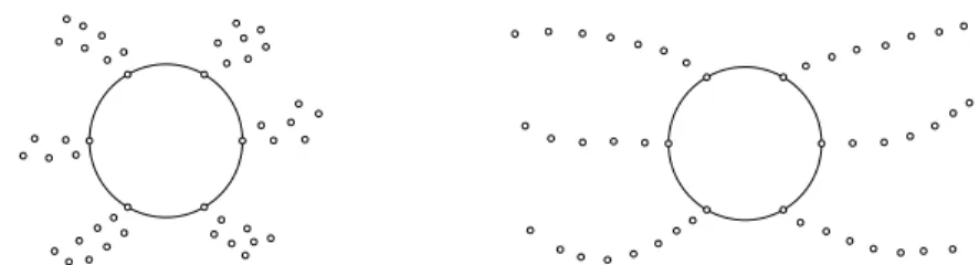
points lie in a cycle that define the flower’s core. When the iterates approach the core along well defined directions we say that the flower is a dandelion.
Figure 2 – A flower and a dandelion with six petals. The dots outside the circles represent the iterates. They accumulate at the points at the circles, which are not critical points of f.
In sections 2 and 7 we present concrete examples of dandelions, for Newton’s method and the BFGS method, respectively. In these examples the line searches are exact, the first Wolfe condition is satisfied and the restrictions of the objective functions to the search lines are strictly convex, the level sets of f are compact, but yet the iterates have the cyclic asymptotic behavior illustrated in Figure 1. The BFGS and Newton’s methods are among the most important line search methods and our examples refute the following conjecture:
If when applying the BFGS or Newton’s methods we choose the first local minimizer along the search line then the iterates converge to a local minimizer of the objective function.
Besides symmetries, this work is based on a theorem proved by H. Whitney in 1934 [17]. Whitney’s theorem regards the extension ofCm functions from subsets ofRn toRn. It says that if a function F and its partial derivatives up
to ordermare defined in a subset E ofRn andF’s Taylor series up to orderm behave properly inEthenFcan be extended to aCm function inRn. Whitney’s theorem is a handy tool to highlight the weak points of nonlinear programming algorithms.
at our disposal increases. We are then able to observe phenomena contrary to our 2 or 3 dimensional intuition. However, as the experience with Lax Pairs has shown [3], “exploiting symmetry” is easier said than done. The algebraic ma-nipulations necessary to implement our ideas can be overwhelming. Although the example for Newton’s method presented in section 2 is a direct consequence of symmetry, we would not be able to build the example for the BFGS method in section 7 without the software Mathematica. Fortunately, today we have the luxury of tools like Mathematica and can focus on the fundamental geometrical aspects of the line search methods.
Our arguments can be adapted to objective functions with mth order Lips-chitz continuous derivatives or to the more general classClocm,ω(Rn)of functions
discussed by C. Fefferman in [7], but we do not aim for utmost generality and restrict ourselves to objective functions with Lipschitz continuous second order derivatives, so that we can speak in terms of gradients and Hessians and avoid the use of higher order multilinear forms. On the other hand, [1] indicates that things are different for analytic objective functions, mainly because these functions are “rigid” and it is not possible to change them only locally, or more technically, due to the lack of analytic partitions of the unity.
This work has six more sections and an appendix. Section 2 motivates our approach by using it to analyze the convergence of Newton’s method. The technical concepts that formalize our arguments are presented in sections 3 and 4. Section 5 discusses the Wolfe conditions and section 6 explains how to build examples in which the objective function is convex along the search lines. In section 7 we combine the results from the previous sections to build an example of divergence for the BFGS method. In the appendix we prove our claims.
may not be able to explain the practical behavior of nonlinear programming algorithms. The main advice one can extract from this work is the following rule of thumb:
If you find that it is difficult to prove that a line search method converges under certain conditions, and other people have tried the same for a couple of decades and did not succeed, then consider the possibility that in theory the method may actually fail under these conditions, even if all your numerical experiments indicate that it always converge.
2 Newton’s method
We now describe a family examples of divergence for Newton’s method for minimization. The examples are parameterized by the step sizeα: givenα >0 we build an example in which all step-sizes αk are equal to α. This section
motivates the theory presented later on. Although the geometry underlying the examples is accurately described by Figure 1, the algebraic details make they look more complex than they really are. Thus, we suggest that you pay little attention to the formulae and focus on the structure of our argument, which can be summarized as follows:
(a) we guess general expressions for the iterates xk, function values fk,
gra-dients gk and Hessianshk which we believe to be compatible with the
symmetries in Newton’s method and the theory presented below.
(b) we plug these expressions into the formula that define Newton’s method and obtain equations relating our guesses in item (a).
(c) we solve these equations and the next sections guarantee the existence of an objective functionF such thatF(xk)= fk,∇F(xk)=gk,∇2F(xk)=hk
andsk∇t 2F(xk+wsk)sk >0 forw∈Randk big enough.
iteratesxk, function values fk, gradientsgk and Hessianshkof the form1: xk = QkD(λk)x, fk = λkf, (10) gk = λkQkD(λ−k)g, hk = λkQkD(λ−k)h D(λ−k)Q−k, (11)
forλ∈(0,1), x =(xh,xv)andg=(gh,gv)withxh,xv,ghandgv ∈R3and
Q =
Qh 0
0 Qv
, D(λ)=
I 0
0 λI
, h=
A C Ct 0
, (12)
whereI is the 3×3 identity matrix, QhandQvare 3×3 orthogonal matrices,
Ais a symmetric 3×3 matrix andCis a 3×3 matrix. We then concluded that
λ= 1
2, x
h
=xv= 1 0 1 ,
Qh =
1 2 √
3 −1 0
1 √3 0
0 0 −2
, Qv=
0 −1 0
1 0 0
0 0 1
(13)
are convenient: they are simple and after picking them we still have the freedom to chooseg, AandC in order to satisfy the hypothesis of the theory presented in the next sections and obtain iteratesxk which are consistent with the formula
∇2F(x
k)sk+α∇F(xk)=0 (14)
that defines Newton’s method with step-size α. If we replace ∇F(xk) and ∇2F(x
x) in (14) by gk andhk in (11) then λ, Qh and Qv cancel out and we
obtain the equations
Ash+Csv+αgh=0, and Ctsh+αgv=0, (15)
1The matricesh
k are not positive definite and in practice one would take another search
direction if, for example, this fact was detected during a Cholesky factorization ofhk. However,
to keep the algebra as simples as possible, in this work we do not enforce the condition that the Hessians∇2f(x
k)are s.p.d. In [14] we show that Newton’s method may fail even∇2f(xk)is
where
sh =(Qh−I)xh and sv=(λQv−I)xv. (16)
Notice that, due to the invariance of Newton’s method with respect to orthogonal changes of variables and scaling, there is no “k” in(15)–(16). Equations (15) yields
gv = −Ctsh/α (17) Equations (10) and (11) show thatsktgk =2−kstg,sktgk+1=2−(k+1)stD(2)Qg,
and fk+1− fk = −2−(k+1)f. Therefore, if
stg<0, stD(2)Qg=0 and f >0 (18) thensk =xk+1−xkis a descent direction, the line searches are exact (sktgk+1=0)
and the first Wolfe condition
fk+1− fk ≤σsktgk
holds for
0< σ <min 1, −f/(2stg).
We now apply the results from the next sections: items 4c and 4d in the definition of seed in section 4 require that
gh=C xv and f =(gv)txv (19) and section 6 says that to guarantee the convexity of the objective function along the search lines we should ask for
2stg<−f <0, sths >0 and stQ D(2)h D(2)Qts >0. (20) To complete the specification of the terms in(10)–(11)we chose the 9 entries ofC and the 6 independent entries of A in order to satisfy(15)–(20). These equations and inequalities are linear in A and C and the following matrices satisfy them:
A=(2+√3)
(2+√3)
17−22α+16α2
2α 2(α−1)
2α (2+√3)(2α−1) 0
2(α−1) 0 0
,
C=(2+√3)
3α−5α2−4 1−α+3α2 α(1+5α)
0 2−√3 0
2−√3 0 0
.
Equations (10)–(13), (16)–(19) and (21) define iterates and function values, gradients and Hessians of the objective function at them. The next sections guarante the existence of an objective function F with Lipschitz continuous second order derivatives such thatF(xk)= fk,∇F(xk)=gkand∇2F(xk)=hk.
Moreover, neither the vectors D′(0)x and D′(0)s nor the vectors D(0)s and
D(0)D(2)s are aligned2and the linesᑦk
= {D(0)xk+wD(0)sk, w ∈ R}are
such thatᑦr ∩ᑦk = ∅for allr +1<k <r +5 and theorem 3 and lemmas 1 and 3 in the following sections show that we have much freedom to chose the value ofF(x)along the search segments{xk+wsk, w∈ [0,1]}: if the function ψ: [0,1] →Rhas Lipschitz continuous second order derivatives and
ψ(0)= f, ψ (1)= f/2, ψ′(0)=gts, ψ′(1)=0, ψ′′(0)=sths, and ψ′′(1)=stQ D(2)h D(2)Qts/2 then F can be chosen so that F(xk +wsk) = (1/2)kψ (w)forw ∈ [0,1] and k large. In fact, condition (20) and theorem 4 in section 6 show that F can be chosen so thatst
kF(xk+wsk)sk >0 forw∈Randklarge and the level sets
(f,z)= x ∈Rn such that f(x)≤ z
are bounded.
3 Flowers and Dandelions
We now present a framework to apply Whitney’s theorem to study the conver-gence of line search methods. We describe examples in which the iteratesxk
and the function values fk, the gradientsgkand the Hessianshk of the objective
function are grouped intopconverging subsequences, which we callpetals(see Figure 2). The limits of these subsequences{xk},{fk},{gk}and{hk}are the
mem-bers of periodic sequences{χk},{ϕk},{γk}and{θk}, so that limq→∞xpq+r =χr
for allr andχr+p=χr, limq→∞ fpq+r =ϕr for allr andϕr+p=ϕr,γr+p=γr
andθr+p =θr. In formal terms:
Definition 1. A flowerF(n,p, λ,xk, fk,gk,hk)is a collection formed by
1. λ∈(0,1)and positive integers n and p.
2. Sequences{xk}and{χk}inRnand a constant M >0such that
(a) xi =xj ⇔i = j .
(b) χj =χk ⇔ j ≡k modp.
(c) λk ≤ Mxk−χk ≤M2λk.
3. Sequences{fk},{ϕk} ⊂R,{gk},{γk} ⊂Rnand{hk},{θk} ⊂Hnsuch that ϕk+p=ϕk, γk+p=γk, θk+p = θk, (22)
hk−θk ≤ Mλk, (23)
gk−γk−θk(xk−χk) ≤ Mλ2k, (24)
fk−ϕk−γkt(xk−χk)−
1
2(xk−χk)
t
hk(xk−χk) ≤ Mλ3k (25) whereHnis the set of n×n symmetric matrices.
Notice that the mod in item 2.b and equation (22) in the definition above imply that the sequences{χk},{γk}and{θk}have period pand item 2.c implies
that ask → ∞the sequence xk accumulates at the limit cycle defined by the χk. The next definitions and theorems relates the fk,gkandhk in a flower to an
objective functionF with Lipschitz continuous second derivatives:
Definition 2. Suppose U ⊂ Rn and V
⊂ Rp. We defineLipm(U,V)as the space of functions F :U → V with Lipschitz continuous mth derivatives. If V =Rthen we call this space simply byLipm(U).
The class LC2(Rn)is interesting because if f ∈ LC2(Rn)then there exists a constantDf such that
f(x)≥ 1
2Cf
x2−Df and ∇f(x) ≥
1
Cf
x −Df.
As a consequence, the level sets
(f,z)= x ∈Rn such that f(x)≤z
are compact, as required by many theorems regarding the convergence of line search methods, and all pointsx with∇f(x) = 0 are such thatx ≤ DfCf.
Thus, the elements of LC2(Rn)have a compact set of critical points and if an
algorithm fails to find one of them then the algorithm is to be blamed, not the objective function. The next theorem shows that flowers can be interpolated by functions in LC2(Rn):
Theorem 2. Given a flowerF(n,p, λ,xk, fk,gk,hk)there exists F ∈LC2(R) such that F(xk)= fk,∇F(xk)=gkand∇2F(xk)=hkfor all k.
If the flower is adandelion then we can improve this result and specify the objective function and its derivatives along the segments{xk+wsk, w ∈ [0,1]}:
Theorem 3. If the functions{Fk},{Gk}and{Hk}and the intervals{[ak,bk]} are compatible with the dandelionD(m,n,p, λ,xk, fk,gk,hk)then there exists k0∈Nand F ∈LC2(Rn)such that F(x
k+wsk)= Fk(w, λk),∇F(xk+wsk)= Gk(w, λk)and∇2F(xk+wsk)= Hk(w, λk)for k >k0andw∈ [ak,bk].
This theorem will make sense after you read the following definitions:
Definition 4. A flower F(n,p, λ,xk, fk,gk,hk) is a dandelion if there exist functions Xk ∈Lip2([0,1],Rn)such that, for all k and Sk(z)= Xk+1(z)−Xk(z),
(a) Xk+p= Xk and xk =Xk(λk).
(b) The vectors Sk(0), X′k(0)and Xk′+1(0)are linearly independent.
Definition 5. The intervals[ak,bk], defined for k ∈N, are compatible with a dandelion if
(a) ak =ak+p ≤0and bk+p=bk ≥1for k ∈N.
(b) The segments{Xk(0)+wSk(0), w ∈ [ak,bk]}and{Xr(0)+wSr(0), w∈ [ar,br]}are disjoint if r+1<k <r+ p−1.
Definition 6. For all k ∈N, consider functions Fk ∈Lip2(R2), G
k ∈Lip1(R2,
Rn)and Hk ∈ Lip0(R2,Hn). We say that{Fk},{Gk}and{Hk}are compatible
with a dandelionDif Fk+p= Fk, Gk+p=Gkand Hk+p= Hk and there exists k0such that if k>k0, i ∈ {0,1},w∈Rand z =λk then
Fk(i,z)= fk+i, Gk(i,z)=gk+i, Hk(i,z)=hk+i, (26) ∂Fk
∂w(w,z)=Gk(w,z) t
sk,
∂Fk
∂z (w,0)=Gk(w,0) t
Vk(w), (27)
∂2F k
∂z2 (w,0)= ∂Gk
∂z (w,0) t
Vk(w)+Gk(w,0)tUk(w), (28) ∂Gk
∂w(w,z)= Hk(w,z)sk,
∂Gk
∂z (w,0)= Hk(w,0)Vk(w) (29) for Vk(w) = (1−w)Xk′(0)+wXk′+1(0) and Uk(w) = (1−w)Xk′′(0)+
wX′′k+1(0).
If we do not care about the derivatives ofFin directions normal to the segments
{xk+wsk, w ∈ [0,1]}then the search for compatible functions Fk,Gkand Hk
is simplified by the following lemma
Lemma 1. LetD(m,n,p, λ,xk, fk,gk,hk)be a dandelion and, for k ∈ N, functions Fk ∈Lip2(R2)for which Fk+p =Fk. If there exist k0∈Nsuch that
Fk(i, λk)= fk+i,
∂Fk ∂w(i, λ
k
)=gkt+isk,
∂2F k ∂w2(i, λ
k
)=skthk+isk (30)
Therefore, we can focus on Fk(w,z)and neglect Hk(w,z)andGk(w,z)for w ∈ {0,1}. In the next section we describe a class of dandelions for which we can restrict ourselves to functionsFk of the formFk(w,z)=zdnψk(w).
4 Symmetric dandelions and their seeds
In this section we present a family of dandelions that includes the examples for the BFGS and Newton’s methods mentioned in the introduction. These dande-lions combine symmetries imposed by an orthogonal matrixQwith contractions dictated by a diagonal matrixD. They are defined by theirseeds:
Definition 7. A seedS(n,p,d,Q,xk, fk,gk,hk)is a collection formed by
1. n, p∈Nand d=(d1. . .dn)∈Nnsuch that p
≥3and dn=maxdi.
2. A n×n orthogonal matrix Q such that Qp = I and the diagonal matrix D(z)with i th diagonal entry equal to zdi commutes with Q for z∈R.
3. A sequence{xk} ⊂ Rnsuch that xk+p = xk, the pointsχr = D(0)Qrxr are distinct for0≤r < p and the vectors
sk = D(λ)Qxk+1−xk (31) are such that, for0 ≤ r < p, the vectors D′(0)xr and D′(0)sr are not aligned and neither are the vectors D(0)sr and D(0)sr+1.
4. Sequences{fk} ⊂R,{g
k} ⊂Rnand{hk} ⊂Hnsuch that
(a) fk+p = fk, gk+p=gk and hk+p =hkfor all k.
(b) (hk)i j =0if di +dj >dn.
(c) If dl =dn−1and J = {j|dj >0}then (gk)l =
j∈J
(hk)l j(xk)j. (32)
(d) If dn ≤ 2, L = {l |dl = dn} and S = {(i, j) |di +dj = dn, di >0, dj >0}then
fk =
l∈L
(gk)l(xk)l +
1 2
(i,j)∈S
A seed andλ∈(0,1)generate a dandelion through the formulae
Xk(z)= QkD(z)xk, xk =Xk(λk), χk = Xk(0), (34) fk =λkdn fk, ϕk =0, (35) gk =λkdnQkD(λ−k)gk, γk =Qkgk∞, (36) hk =λkdnD(λ−k)QkhkQ−kD(λ−k), θk =Qkh∞k Q−
k, (37)
where
(gk∞)i =(gk)i if di =dn and (gk∞)i =0 otherwise, (38) (h∞k )i j =(hk)i j if di+dj =dn and (h∞k )i j =0 otherwise. (39)
This result is formalized by the following lemma:
Lemma 2. IfS(n,p,d,Q,xk, fk,gk,hk)is a seed andλ∈ (0,1)then there exists a unique dandelionD(S)with Xk, fk, gk, hk,ϕk,γkandθkas in(34)–(39). Moreover,D(S)’s steps sk =xk+1−xkare given by
sk = QkD(λk)sk (40)
for sk defined in(31).
It is easy to apply lemma 1 and theorem 3 toD(S):
Lemma 3. If S(n,p,d,Q,xk, fk,gk,hk) is a seed, λ ∈ (0,1), xk, fk, gk and hk are given by (34)–(37) and the functions ψr ∈ Lip2(R), defined for
0≤r < p, satisfy
ψr(i)= fr+i, ψr′(i)=s t
rgr+i, ψr′′(i)=s t
rhr+isr (41) for i ∈ {0,1}then the functions Fk(w,z)=zdnψkmodp(w)satisfy(30).
To build a symmetric dandelion and specify the value of the objective function along the search segments{xk+wsk, w ∈ [0,1]}it is enough to find the right
F with∇F(xk) = gk,∇2F(xk) = hk and F(xk +wsk) = λkdnψkmodp(w)for xk, fk,gk andhk in(34)–(37)is guaranteed by lemma 3 and theorem 3. To find
a seed we proceed as in section 2: we plug(34)–(37)into the expressions that define
(a) the method of our interest,
(b) the compatibility conditions in the definition of seed and theorem 3,
(c) additional constraints, like the Wolfe conditions in section 5 and the convexity conditions in section 6.
and analyze the result. If equations(34)–(37)are compatible with the method’s symmetries, as they are for the BFGS and Newton’s methods, then we have a chance of handling these constraints and may even find closed form solutions for them. If equations(34)–(37)are not related to the method’s symmetries then the dandelion will not bloom.
5 The Wolfe conditions
In this section we show that the Wolfe conditions
fk+1− fk ≤σgktsk (42)
and
sktgk+1≥βgtksk (43)
may not prevent the cyclic behavior illustrated in figures 1 and 2. In fact, we can have cyclic behavior even if we replace the second Wolfe condition(43)by the stronger requirementsktgk+1 = 0, which is called exact line search condition.
These conditions are invariant with respect to orthogonal changes of variables and scaling and can be easily checked for the dandelions coming from a seed:
Lemma 4. LetS(n,p,d,Q,xk, fk,gk,hk) be a seed andD(m,n,p, λ,xk, fk,gk,hk)the corresponding dandelion.
(b) If strgr <0 for 0≤r < p then the first Wolfe condition(42)holds for
σ < σ0= min
0≤r<p
λdn f
r+1− fr strgr
.
(c) If srtgr < 0 for 0 ≤ r < p then the second Wolfe condition(43) is verified for
β > β0= max
0≤r<p strgr+1
srtgr
.
6 Convexity along the search lines
Convexity is an important simplifying assumption in optimization. It is tempting to conjecture that strict convexity along the search lines guarantees the conver-gence of line search methods3. Sometimes even stronger conjectures are made, like having convergence if we choose a global minimizer or the first local mini-mizer along the search line. We now show that strict convexity along the search lines does not rule out the cyclic behavior depicted in figures 1 and 2. To do that, we present a theorem that yields an objective function which is strictly convex along the search lines of a dandelion that comes from a seed:
Theorem 4. Let S(n,p,d,Q,xk, fk,gk,hk) be a seed, λ ∈ (0,1) and xk, χk, fk, gk and hk be given by(34)–(37). Letᑥbe the convex hull of{χk,0 ≤ k ≤ p}. Consider the linesᑦk = {χk+w(χk+1−χk), w ∈R}and assume that ᑦr ∩ᑦk∩ᑥ= ∅for r+1<k<r +p−1. If, for0≤r < p,
srtgr < fr+1− fr <srtgr+1, srthrsr >0 and srthr+1sr >0 (44) then there exist a function F∈LC2(Rn)and k0such that if k >k0then F(xk)=
fk,∇F(xk)=gk,∇2F(xk)=hk and skt∇2F(xk+wsk)sk >0for allw∈R.
the objective function is strictly convex along the search lines we can focus on (44) and check the intersections later, just to make sure we were not unlucky. This is what we did in section 2 and will do again in the next section.
7 The BFGS method
In this section we present an example of divergence for the BFGS method in which the objective function is strictly convex along the search lines. The essence of this example is already present in [13] and we suggest that you read this reference as an introduction to this section. Our purpose here is to show that the concepts of flower, dandelion and seed reduce the construction of examples like the one in [13] to the solution of algebraic problems. Software like Mathematica or Mapple can decide if such algebraic problems have solutions and find accurate approximation to these solutions. The validation of the example becomes then a question of using these approximate solutions wisely to check the requirements in the definitions of flower, dandelion and seed and the hypothesis of the lemmas and theorems in the previous sections.
We analyze the BFGS method with exact line searches, i.e., sktgk+1 = 0. In
this case the Hessian approximationsBkare updated according to the formula:
Bk+1=Bk+ αk sktgk
gkgtk−
1
sktgk
(gk+1−gk)(gk+1−gk)t, (45)
wheregk = ∇F(xk). The iteratesxk evolve according to
sk = −αkBk−1gk and xk+1=xk+sk. (46)
Equations(45)–(46)are invariant with respect to orthogonal changes of variables and scaling, in the sense that if Q is an orthogonal matrix, λ ∈ R and F, Bk andxksatisfy equations(45)–(46)thenF(x)=F(λ−1Qtx),Bk =λ−2Q BkQt
andxk =λQxk satisfy them too. It is hard to exploit these symmetries because
the BFGS method was conceived to correct the matrices Bk. However, it has an
additional symmetry: if we takeBkof the form
Bk = − n−1
i=0 αk+i gkt+isk+i
combined with the conditions
sktgk <0 and sktgk+j =0 for 1≤ j<n and k ∈N, (48)
then equation (46) is automatically satisfied and (45) holds if
gk+n=ρk(gk+1−gk), (49)
forρksuch that
αk+n=
skt+ngk+n st
kgkρk2
. (50)
Notice that if we assume (48) and takeαk = 1 for 0 ≤ k < n,αk in (50) for k ≥ n then theαk are positive and the vectorsgk, . . .gk+n−1are linearly
inde-pendent, because if we suppose thatnj−=10µjgk+j =0 withµ0 =1 then (48)
leads to the contradiction 0 = st k
n−1
j=0µjgk+j = sktgk < 0.Therefore, under (48)–(50)the matrices Bk defined by(47)are positive definite and to build an
example of divergence for the BFGS method we can ignoreαk andBkand focus
on(48)–(49).
To apply the theory above we plug(34)–(37)into (48) and (49) and deduce that a seedS(n,p,d,Q,xk, fk,gk,hk)is consistent with the BFGS method if
stkgk <0 and stkD(λ− j)Qjg
k+j =0 for 1≤ j <n, (51) Zngk+n =ρk
Z gk+1−gk
, (52)
whereZ =λdnD(λ−1)Q. If we fixZthen (52) becomes similar to an eigenvalue
problem, with theρ’s playing the role of eigenvalues and theg’s of eigenvectors. We solved equations (52) forgk andρkin the case
Q=
cos33π −sin33π sin33π cos33π
−1 1 −1 1
, D(λ)= 1 1 1 λ λ λ3 ,
Lemma 5. If Q and D(λ)are the matrices above, dn =3, n =6andλ= 11 √
0.9
then there exist vectors gk ∈ R6 and coefficients andρ
k ∈ Rthat satisfy(52) and are such that gk+11 =gk,ρk+11 =ρk and the six vectors in the set
D(λ−j)Qjgk+j, j =0,1, . . . ,5
(53)
are linearly independent for each k∈N. The linear independence of the vectors D(λ−j)Qjg
k+j in lemma 5 implies
that we can solve the following linear systems of equations on the vectorssk: stkgk = −1 and stkD(λ−
j)Qjg
k+j =0 for 1≤ j <6. (54)
The vectorsskobtained from (54) define stepssk by (40): sk =Xksk for X = D(λ)Q
and we claim that the points
x0 = −I −X11−1 10
j=0
Xjsj, (55)
xk = X−k
x0+ k−1
j=0 Xjsj
for k >0 (56)
satisfy
xk+66 =xk (57)
and lead to pointsxk = Xkxk such thatsk = xk+1−xk. In fact, using (56) it
is straightforward to deduce thatxk+1−xk = Xk+1xk+1−Xkxk = Xksk =sk.
To verify (57), notice that (56) yields
xk+66 = X−k
x0+ k+65
j=66
Xj−66sj+X−66
(58)
where
=I −X66x0+ 65
j=0
Now, sincegk+11=gk, equation (54) implies thatsk+11 =skand 65
j=0
Xjsj = 5
r=0 X11r
10
j=0
Xjsj =(I −X11)−1(I −X66) 10
j=0 Xjsj.
Combining this equation, (55) and (59) we conclude that = 0 and equation
(58) and the identitysj−66 =sj lead to (57).
In the proof of lemma 5 we show that thegkcan be chosen so that the vectors skdefined by (54) satisfy the linear independence requirements in the definition
of seed. Thexk andgkabove,d =(0,0,0,1,1,3),
fk =1 and hk = D′(0)skstkD′(0) (60)
are also compatible with this definition. As a consequence,n = 6, p =66,d,
Q xk,fk,gk andhk define a seedS. This seed leads to a dandelion D(S) with
stepssk and gradients gk compatible with the BFGS method with the matrices Bkin (45) and step sizesαkin (50). Equations(34)–(37)and (54) imply that the
function values and gradients associated toD(S)satisfy
sktgk = −λ3k < λ3k+3−λ3k = fk+1− fk <0=sktgk+1. (61)
Lemma 4 shows that the iterates xk corresponding toD satisfy the first Wolfe
condition for 0 < σ < 1−λ3. Moreover, almost all choices of the vectorsgk
in the proof of lemma 5 lead to linesᑦk = {D(0)Qkx
k+wD(0)Qksk, w∈R}
such thatᑦr ∩ᑦk = ∅forr +1<k <r+65 andsktD′(0)sk+1 =0. Equation
(60) shows thatskthksk > 0 and skthk+1sk > 0. As a result, equation (61) and
theorem 4 yield an objective function F ∈ LC2(R6) such that the iterates xk generated by applying the BFGS method toFwithx0=x0andBkabove satisfy skt∇2F(xk+wsk)sk >0 forklarge andw∈R.
This completes the presentation of an example showing that there is not enough strength in the definition of the BFGS method, the exact line search condition and the Wolfe conditions to prevent the cyclic behavior in figures 1 and 2, even when the objective function is strictly convex along the search lines and has compact level sets.
the eigenvalue problem (52) does not seem to have real solutionsρk = 0 for n<6. Notice that this is a purely algebraic issue, which has nothing to do with nonlinear programming. Similarly, the minimum dimension at which we could build counter examples with the techniques described here for other methods could be bigger or smaller than 6, depending on the particular symmetries of the method and the existence of solutions for the corresponding algebraic problems.
8 Appendix
We now prove the results stated in the previous sections. Our main tool is the following corollary of the Whitney’s extension theorem:
Lemma 6. Let E be a bounded subset of Rn and suppose F : E → R, G : E → Rn and H : E → Hn are functions with domain E and M is a
constant. If
H(x)−H(y) ≤My−x, (62)
G(y)−G(x)−H(x)(y−x) ≤ My−x2, (63)
|F(y)−F(x)−G(x)t(y−x)−1
2(y−x)
tH(x)(y −x))|
≤ My−x3 (64)
then there exists F ∈ Lip2(Rn) such that F(x) = F(x),∇F(x) = G(x)and
∇2F(x)=H(x)for x ∈ E . Moreover, there exists constants C and R such that ifx ≥ R then∇2F(x)is positive definite and∇2F(x)−1 ≤R.
Whitney’s theorem is stated in different levels of generality in the pure mathe-matics literature. The most complete and general approach is due to C. Fefferman [7, 8] but, unfortunately, it is stated in a language that is too abstract for the av-erage non linear programming researcher. In page 48 of [10], L. Hörmander presents a more concrete version of the theorem for functions inCm. This
ver-sion of the theorem is stated usingn-uples to denote partial derivatives, i.e., if
α=(α1, . . . , αn)∈Nn,|α| =αi and f is a function with partial derivatives
of order|α|then∂αf(x)is defined as
∂αf(x)= ∂
α1∂α2. . . ∂αk
∂xα1
1 ∂x
α2
2 . . . ∂x
αk n
Moreover,α! =
αi andxα =
xαi. Using this notation, the arguments used
to prove theorem 2.3.6 in [10] can be adapted to prove the following version of Whitney’s theorem:
Theorem 5. Let E be a bounded set inRnand consider, for eachα ∈Nnwith |α| ≤m, a Lipschitz continuous function uα :E →R. If there exists a constant
M such that
uα(x)−
|β|≤m−|α| 1
β!uα+β(y)(x−y)
β
≤ Mx−ym−|α|+1
for all x,y ∈ E andα∈Nnwith
|α| ≤m then there exists f ∈Lipm(Rn)such that∂αf(x)=u
α(x)for allα ∈Nnwith|α| ≤ m and x ∈ E . Moreover, there
exists a constant C such that|∂αf(x)| ≤ C for all x ∈ Rn andα ∈ Nn with
|α| ≤m.
This theorem allows us to extend much of the discussion in this work to Lipm(Rn)form >2. However, form > 2 we cannot group the partial
deriva-tives in vectors (gradients) and matrices (Hessians) as we did in the statement of lemma 6. As a consequence, the geometry behind the examples gets blurred by the technicalities asm increases and we decided it would be best to focus on the consequences of lemma 6 instead of exploring more general results like theorem 5.
We can apply Whitney’s result to a dandelionDwithxk =Xk(λk)because if Sk(z)= Xk+1(z)−Xk(z), Xk(w,z)= Xk(z)+wSk(z) (65)
andδ > 0 is small and the intervals{[ak,bk]} are compatible withD then the
distance between points in the 2 dimensional surface
∞
k=0
Xk(w,z), w ∈ [ak,bk] and z ∈ [0, δ]
Lemma 7. Given a dandelion with xk = Xk(λk), compatible intervals{[ak, bk]} and Xk in(65)there existsδ > 0such that ifwj, wk ∈ [ak,bk], zj,zk ∈ [0, δ], yj =Xj(wj,zj), yk =Xk(wk,zk)andyj −yk ≤δthen either
(a) j ≡k mod p, (b) j ≡k+1 mod p or (c)k ≡ j+1 mod p (66)
and in case (a)
yj−yk ≥δ
|wj−wk| + |zj−zk|
, (67)
in case (b)
yj −yk ≥δ
|wj| + |zj −zk| + |1−wk|
(68)
and in case (c)
yj−yk ≥δ
|1−wj| + |zj −zk| + |wk|
. (69)
We also use the next lemmas. After the statement of these lemmas we prove the theorems and the paper ends with the proofs of the lemmas.
Lemma 8. Consider E ⊂Rn, constants K >1,δ >0and functions F : E → R, G : E →Rn and H
: E → Hn. If for all x,z
∈ E there exist m ∈ Nand
y1, . . . ,ym ∈ E such that, for y0=x and ym+1=z, m
i=0
yi+1−yi ≤Kx −z, (70)
H(yi)−H(yi+1) ≤ Kyi+1−yi, (71) G(yi+1)−G(yi)−
1
2(H(yi+1)+H(yi))(yi+1−yi)
≤Kyi+1−yi2, (72)
F(yi+1)−F(yi)−
1
2(G(yi+1)+G(yi))(yi+1−yi)
≤Kyi+1−yi3, (73)
Lemma 9. If the dandelion D(m,n,p, λ,xk, fk,gk,hk) and the functions {Fk},{Gk}and{Hk}are compatible and the equations(26)–(29)hold for k>k0 then there exists M ∈Rsuch that if j,k >k0and u, w ∈Rthen
Hk(u, λk)−Hk(w, λk) ≤M|u−w|, (74) Gk(u, λk)−Gk(w, λk)−
1
2(Hk(u, λ
k)
+Hk(w, λk))h
≤ M|u−w|2, (75)
Fk(u, λk)−Fk(w, λk)−
1
2(Gk(u, λ
k)
+Gk(w, λk))th
≤ M|u−w|3, (76)
Hk(w, λj)−Hk(w, λk) ≤ M|λk−λj|, (77) Gk(w, λj)−Gk(w, λk)−
1
2(Hk(w, λ
j)
+Hk(w, λk))v
≤ M|λk−λj|2, (78)
Fk(w, λj)−Fk(w, λk)−
1
2(Gk(w, λ
j
)+Gk(w, λk))tv
≤ M|λk−λj|3, (79)
for h = Xk(u, λk)− Xk(w, λk), v = Xk(w, λj)− Xk(w, λk) and X as
in(65).
Lemma 10. If f0, f1, g0, g1, h0and h1∈Rare such that g0< f1− f0<g1,
h1 > 0 and h2 > 0 then there exists ψ ∈ Lip2(R) such that ψ (0) = f0,
ψ(1)= f1,ψ′(0)=g0,ψ′(1)=g1,ψ′′(0)=h0,ψ′′(1)=h1andψ′′(w) >0
for allw∈R.
Lemma 11. Given a function ψ ∈ Lip1(R2) such that ψ (i,0) = 0 and
∇ψ(i,0)=0for i∈ {0,1}there existsφ ∈Lip1(R2)such that (a) φ(i,z)=0 and ∇φ(i,z)=0 for i ∈ {0,1} and z ∈R.
Lemma 12. Considerλ∈ (0,1), a function F ∈ Lip2(R2), functions Y1and
Y2inLip2([0,1],Rn)and Y3(z)=Y2(z)−Y1(z). If the vectors Y′
1(0), Y2′(0)and Y3(0)are linearly independent and, for i ∈ {0,1},
F(i,0)=0, ∇F(i,0)=0 and ∇2F(i,0)=0 (80)
then there existδ > 0, G ∈ Lip1(R2,Rn)and H ∈ Lip0(R2,Hn)such that if
z ∈ [0, δ]and i ∈ {0,1}then
G(i,z)=0, G(w,z)tY3(z)= ∂F ∂w(w,z), G(w,0)tV(w)= ∂F
∂z(w,0),
(81)
∂G ∂z(w,0)
tV(w)
+G(w,0)tU(w)= ∂ 2F
∂z2(w,0), (82) H(i,z)=0, H(w,z)Y3(z)= ∂G
∂w(w,z), H(w,0)V(w)= ∂G
∂z (w,0)
(83)
for
V(w)=(1−w)Y1′(0)+wY2′(0) and
U(w)=(1−w)Y1′′(0)+wY2′′(0).
Proof of Theorem 2. Item 2 in the definition of flower in section 3 implies that there existsδ > 0 such that if xk −xj ≤ δ then j ≡ k mod p. The
periodicity ofϕk,γk andθkgiven by (22), item 2 in definition 1 and the bounds
(22)–(25) imply that ifxandzbelong to the setE = {xk, k ∈N} ∪ {χk, k ∈N}
andx −z ≤δ then there existsk such thatm =1 and y1 = χk satisfy the
conditions (70)–(73) in lemma 8. Therefore, lemmas 6 and 8 imply that there
exists a functionF as required by theorem 2.
Proof of Theorem 3. Considerk0andδobtained from lemma 7 and
E =
∞
k=k0
Xk(w, λk), w ∈ [ak,bk]
Lemma 7 and the three equations in (26) imply that the expressions
F(Xk(w, λk))= Fk(w, λk), G(Xk(w, λk))=Gk(w, λk), H(Xk(w, λk))= Hk(w, λk)
define functions F,Gand H with domainE, i.e., if Xj(wj, λj)= Xk(wk, λk)
then
Fj(wj, λj)=Fk(wk, λk), Gj(wj, λj)=Gk(wk, λk), Hj(wj, λj)= Hk(wk, λk).
Lemmas 7 and 9 show that the functionsF,GandHabove satisfy the hypothesis
of lemma 8 and theorem 3 follows from lemma 6.
Proof of Theorem 4. Forρ >0, consider the compact convex set
ᑥρ = {x ∈Rn| sup
y∈ᑥ
x−y ≤ρ}.
Sinceᑦk∩ᑦr∩ᑥ= ∅forr +1<k<r +p−1 there existsǫ > 0 such that ᑦk∩ᑦr ∩ᑥ2ǫ = ∅for the samekandr. For each 0≤r < pthere existar <0
andbr >1 such that
ᑦr ∩ᑥ2ǫ = {Xr(0)+wSr(0), w∈ [ar,br]}.
Extending the definition ofak and bk by periodicity, ak = akmodp andbk = bkmodp, we obtain intervals[ak,bk]compatible withD. Combining lemmas 1,
3 and 10 and theorem 3 we obtaink1 and F ∈ Lip2(Rn) such that ifk > k1
thenF(xk)= fk,∇F(xk)=gk,∇2F(xk)=hk andskt∇ 2F(x
k+wsk)sk >0 for w∈ [ak,bk].
The pointsXk(0)belong to the interior of the compact convex setᑥǫand there
existck <0 anddk >1 such thatck+p=ck,dk+p=dk and ᑦk ∩ᑥǫ = Xk(0)+wSk(0), w∈ [ck,dk]
and vectorsUk,Vksuch thatUk+p=Uk,Vk+p=Vk,UktSk(0) <0,VktSk(0) >0
and
Ukt(x−Xk(0)−ckSk(0))≤0 and Vkt(x−Xk(0)−dkSk(0))≤0 for x ∈ᑥǫ.
LetLbe a Lipschitz constant for the second derivatives of F,µ >0 such that
µ3
Sk(0)<−UktSk(0) and µ3
Sk(0)<VktSk(0) for k ∈N
andτ :R→Rbe the functionτ (w)=max(w,0)3. The function F(x) = F(x)+ L
µ3 p
r=0
τ (Urt(x−Xr(0)−crSr(0)))
+ τ (Vrt(x−Xr(0)−drSr(0)))
and k0>k1 such that µ√3
sk<−3Uktsk and µ√3 sk<3Vktsk,
Ukt(xk+bksk−Xk(0)−ckSk(0)) >0 and Vkt(xk+bksk−Xk(0)−dkSk(0)) >0
fork >k0are as required by theorem 4. In fact, F coincides withF inᑥǫ and
ifk >k0andw >bk then
skt∂ 2F
∂w2(xk+wsk)sk ≥s t k
∂2F
∂w2(sk+bksk)sk−L(w−bk)sk +6L
µ3(V t
rsk)2Vkt(xk−bksk−Xk(0)−dkSr(0)) +(w−bk)
6L µ3(V
t
rsk)3> L(w−bk)sk.
Proof of Lemma 1. LetF be the function obtained by applying theorem 2 to
D. Lemma 12 applied to the functions F˜ = Fk −F,Y1 = Xk andY2 = Xk+1
yield functions G˜k and H˜k such that Gk(x) = ∇F(x)+ ˜Gk(x)and Hk(x) = ∇2F(x)
+ ˜Hk(x)are as claimed in lemma 1.
Proof of Lemma 2. Equations (34)–(37) show that
Xk(z)= n
j=1 zdj(x
r)jej and gk = n
i=1
λk(dn−di)(g
whereei ∈ Rn is the vector with ei i = 1 andei j = 0 fori = j, Item 4b in
definition 7 implies that ifT = {(i, j)such thatdi +dj ≤dn}then hk =
(i,j)∈T
λk(dn−di−dj)(h
k)i jeietj. (85)
SinceQp =I andx
k+p =xk, the Xkin (34) satisfy item (a) in the definition of
dandelion. The relations fk+p = fk,gk+p =gk andhk+p =hk imply that fk, gk andhk accumulate at the limitsϕk,γk andθkin the last column of (34)–(37)
and these limits satisfy (22). We now verify (23)–(25). Equation (85) yields (23). The first equation in (84) leads to
k =xk −χk =
j∈J λkdj(x
k)j, (86)
whereJ = {j|dj >0}. The second equation in (84) and (85) imply that gk−γk −θk∞k ≤nλk
u∈U
|(gk)u−
j∈J
(hk)u j(xk)j| +O(λ2k) (87)
forU = {u |du =dn−1}and equations (87) and (32) show that thegk satisfy
(24). Equations (38), (39) and (86) lead to
gk∞k =λkdn
j∈G
(gk)j(xk)j and tkθk∞k =λkdn
(i,j)∈T
(hk)i j(xk)i(xk)j,
forL andS in item 4b of definition 7, and (25) follows from (33). Finally, the linear independence requirements in items (b) and (c) of definition 4 follow from
item 3 in definition 7.
Proof of Lemma 3. Direct computation using (34)–(37) and (41) show that
the functionFksatisfies (30).
Proof of Lemma 4. To prove this lemma, plug (34)–(37) into the expressions
Proof of Lemma 5. The matrixZ in (52) can be written as
Z =λ3D(λ−1)Q=
Z1 0 0 0 0
0 Z2 0 0 0
0 0 Z3 0 0
0 0 0 Z4 0
0 0 0 0 Z5
, (88)
where theZi’s are the following 1×1 and 2×2 blocks:
Z1=λ3
cos33π −sin33π sin33π cos33π
, Z2= −λ3, Z3=λ2, Z4= −λ2, Z5=1. (89)
If we identify the blocksZi with the complex numbers
z1=λ3eπ33i, z2= −λ3, z3=λ2, z4= −λ2, z5=1. (90) then (52) can be interpreted as the equations
z6kgˆk+6=ρr
zkgˆj,k+1− ˆgj,k
, (91)
in the complex variablesgˆj,k given by ˆ
g1,k =(gk)1+i(gk)2, g2ˆ ,k =(gk)3, (92) ˆ
g3,k =(gk)4, g4ˆ ,k =(gk)5, g5ˆ ,k =(gk)6. (93)
In the case ρk+11 =ρk and gr+11 =gr equation (91) is equivalent to
A(1/ρ0,1/ρ2, . . . ,1/ρ10,−zj)gˆj =0, (94)
where gˆj =(gˆj,0,gˆj,1,gˆj,2,gˆj,3, . . . ,gˆj,7,gˆj,10)t and
A(y,z)=
1 z 0 0 0 0 y0z6 0 0 0 0 0 1 z 0 0 0 0 y1z6 0 0 0 0 0 1 z 0 0 0 0 y2z6 0 0 0 0 0 1 z 0 0 0 0 y3z6 0 0 0 0 0 1 z 0 0 0 0 y4z6 y5z6 0 0 0 0 1 z 0 0 0 0
0 y6z6 0 0 0 0 1 z 0 0 0 0 0 y7z6 0 0 0 0 1 z 0 0 0 0 0 y8z6 0 0 0 0 1 z 0 0 0 0 0 y9z6 0 0 0 0 1 z z 0 0 0 0 y10z6 0 0 0 0 1
Equation (94) suggests that we takeρ0,ρ1,. . .,ρ10such that the corresponding matrices Ain (95) are singular. Given suchρ’s we can find vectorsgˆj =0 that
satisfy (94) and use them to define the vectorsgtaking real and imaginary parts of (92)–(93). This approach leads to the polynomial equations
det(A(y,−zj))=0 for j=1,2,3,4,5 (96)
on the yr = 1/ρr. To obtain accurate approximations for appropriatedρr we
take
y6= −1.9948, y7= −0.3737, y8= −1.2355, y9=0.9857, y10 =0.11717 and apply Newton’s method to find the remainingyi. Expression (96) correspond
to a system of six real equations and Newton’s method starting with
y0=2.04831, y1=3.33798, y2= −1.15867,
y3=0.300795, y4= −0.634211, y5= −2.44761,
converges quickly to a solution of this system. This approach led to ratio-nal approximations y′s for the yi’s such thatdet(A(y,−zj)) < 10−1000 for j = 1,2,3,4 and 5 and such that the Jacobian of the system (96) is well
con-ditioned at y. A standard argument using Kantorovich’s theorem proves the
existence of an exact y in a neighborhood of radius 10−500 of our rational
ap-proximation. Using the approximation y we dropped the last row in each of
the matrices A(y,−zj)and computed highly accurate approximations for the
five complex vectorsgˆj ∈ R11 in (94) normalized by the condition(gˆj)1 =1. Using (92)–(93) we obtained accurate approximations to the vectorsgjrequired
by lemma 5. Using these approximations we verified that the vectors in (53) are indeed linearly independent and solved the systems (54) for the vectorssk.
Finally, we computed approximations for thexkin (55)–(56) and verified that the
corresponding linesᑦk andᑦr in the hypothesis of theorem 4 are at least 10−5
apart. Our computations indicate that the exact lines ᑦk andᑦr do not cross.
We did a rigorous sensitivity analysis of the computations above and it indicated that 500 digits is precision enough to guarantee that our conclusions apply to the