Hydrophobic Models of Protein Folding
and the Thermodynamics of Chain-Boundary Interactions
Ays¸e Erzan
1,2 1Department of Physics, Faculty of Sciences and Letters
Istanbul Technical University, Maslak 80626, Istanbul, Turkey
2
Feza G¨ursey Institute, P. O. Box 6, C¸ engelk¨oy 81220, Istanbul, Turkey
and Erkan T¨uzel
3 3School of Physics and Astronomy, University of Minnesota, 116 Church St. SE, Minneapolis, MN 55455, USA
Received on 9 May, 2003
We review some results concerning the energetic and dynamical consequences of taking a generic hydrophobic model of a random polypeptide chain, where the effective hydrophobic interactions are represented by Hookean springs. Then we present a set of calculations on a microscopic model of hydrophobic interactions, investigating the behaviour of a hydrophobic chain in the vicinity of a hydrophobic boundary. We conclude with some speculations as to the thermodynamics of pre-biotic functions proteins may have discharged very early on in the evolutionary past.
I
Introduction
The approach of a statistical physicist to biological problems is different from that of a biologist, in the same way that the approach of a physicist to any natural phenomenon is differ-ent from that of an engineer. The difference seems to lie in regarding any given instance of a particular phenomenon not as the product of an ingenious design, but only as a member of a very large ensemble of possible realizations of a generic rule, all governed by the same laws of physics. To a statisti-cal physicist, a biologistatisti-cal molecule is not, first and foremost, a high precision tool custom-made to perform a highly spe-cialized task; it is rather a member of a very large set of pos-sible outcomes of random processes, which, under nonequi-librium conditions, have conspired to produce a certian, al-beit very improbable result. Moreover, as has already been thoroughly underlined by Eigen [1] and Maynard-Smith [2], biological entities typically correspond to sharply peaked probability distributions (“quasispecies”) about some point in biological phase space, rather than unique solutions to some optimization problem. This distribution is of course reflected in the genetic code, and also must translate itself to the proteins that make up the organism.
Another source of deviations from perfect order is ther-mal noise. We would like to stress that the protein in its native state must essentially correspond to a self-organized system, i.e., the “native state” should be concieved of as the attractor of a dynamics [3]. This typically corresponds not to a unique conformation but to a set of conformations to which the trajectory of the phase point representing the molecule is
confined after asymptotically long times (which may already be achieved in microseconds).
In this paper we will first review a simple model in-volving discrete torsional degrees of freedom [3]. The hy-drophobic interactions driving the folding of the polypep-tide chain [4, 5] are modeled by Hookean springs con-necting pairs of hydrophobic residues. [6-12] This sys-tem, with harmonic interactions, under dissipative dynam-ics driven by random noise, leads to a distribution of en-ergy states obeying a modified one-dimensional Ornstein-Uhlenbeck [13, 14] process, quite independently of the na-ture of the sequence of hydrophobic and polar residues, or the dimensionality of the space. It can be shown to obey the so called Wigner distribution [15-19]
P(ǫ)∼ǫ exp(−π
4ǫ
2) ,
(1) over a very large range of energiesǫrelative to someEmin. This distribution resembles that found for the vibrational en-ergy density of real proteins [6].
relaxation path in phase space also obeys a stretched expo-nential form, with another exponenta ≃ 0.39. In [20] we show thatα=a/(a+ 1), which yields a value forαin very good agreement with our simulation results.
In the second part of this review, we would like to dis-cuss work done with Pınar ¨Onder [25], on the statistics of a hydrophobic chain near a hydrophobic boundary. The hy-drophobic interaction arises from the competition between the energy and the entropy terms in the free energy. It turns out that so-called hydrophobic molecules can, in fact, lower the total internal energy when intermixed with the water molecules, but only in a low entropy state of water with a high degree of short range order. For low enough tempera-tures, this state is, in fact, the equilibrium state as it lowers the free energy. However, for somewhat higher tempera-tures, the entropy term in the free energy wins out, and the hydrophobic (non-polar) molecules seperate out from the water molecules, which are now in a completely disordered state. At still higher temperatures, even this segregation dis-appears.
The decorated lattice model proposed by Widom and co-workers [26-31] provides a microscopic basis for the statis-tical physics of the so called hydrophobic interaction, which is an effective, entropy driven phenomenon. We adapted the Widom model to investigate the behaviour of hydropho-bic chains in the neighborhood of hydrophohydropho-bic boundaries. The motivation was to eventually understand the role of hy-drophobic surfaces in the process of protein folding, i.e., to see if they could provide a chaperoning effect. We have been able to treat certain aspects of the problem analytically, by restricting ourselves to two dimensions, and treating the wall-chain interaction in a one-dimensional approximation. Nevertheless the full solution still involves a certain amount of numerical manipulation. It is gratifying to find that within a given temperature interval, the hydrophobic chain prefers to adsorb on a hydrophobic boundary, and outside this in-terval it is more or less in a randomly coiled state. More-over, within this interval, the chain is adsorbed in a more stretched or collapsed configuration, for lower and higher temperatures, respectively, and remains somewhat collapsed at temperatures high enough for it to have just desorbed from the wall. The interplay between the entropy of the water molecules and the entropy of the chain is what gives rise to this nonmonotonic behaviour.
In the last part we will briefly discuss the thermodynam-ics of the folding of hydrophobic or randomly polar and hy-drophobic polypeptide chains near a hyhy-drophobic wall and speculate as to the evolutionary possibilities to which this may have given rise, for the selection of those chains with narrowly defined native states [32].
The paper is organized as follows. In section II, we dis-cuss the energetics and the glassy relaxation behaviour of the simple Hookean model, in section III, we present our results on the hydrophobic chain near a hydrophobic bound-ary, and in section IV, provide a brief summary of a scenario for protein-RNA co-evolution, with prospects for further re-search.
II
A Gaussian model for protein
fold-ing
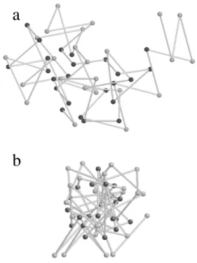
The Gaussian model of a polypeptide chain we consid-ered [3, 20] consisted of a chain of N residues (treated as point vertices), chemical bonds of fixed length along the backbone, and N −3 dihedral angles (see Fig. 1). We assumed that we are in a temperature range where the hydrophobic interactions are appreciably strong. The hy-drophobic interactions between the non-polar residues will then act in such a way as to segregate them from the po-lar residues and the ambient water molecules. We mimick the effective hydrophobic interactions by placing Hookean springs between all pairs of non-polar residues.
a
b
Figure 1. A chain ofN= 48residues, half of which are randomly chosen to be hydrophobic, (darker beads) shown in a random ini-tial and a collapsed configuration in panels (a) and (b) respectively. (Generated using RasMol V2.6)
no “teleological” information that is fed into the system by connecting only thoseH−Hpairs which are close to each other in the native configuration for a particular sequence.
It is known that real proteins are distinguished byH, P sequences that lead to unique ground states while a ran-domly chosen H, P sequence will typically give rise to a highly degenerate ground state. In the absence of detailed knowledge regarding the rules singling out the realisticH, P sequences we considered a genericH, P sequence obtained by choosing fifty percent of the residues to be hydropho-bic and distributing them randomly along the chain. We have checked that our results were quite robust with respect to changing the sequence of hydrophobic or hydrophilic residues, or even taking all of them to be hydrophobic. (In the last section of this paper we will indulge in some specu-lation as to how those sequences with unique ground states may have been selected for.)
In this model, the energy of the molecule is given by
E= K 2
X
i,j
ci,j|ri−rj|2=KX
i,j
r†
iVijrj (2)
If we defineQi = 1for theith vertex being occupied by a hydrophobic residue, andQi = 0otherwise, we may write ci,j=QiQj, and the interaction matrix then becomes
Vij = [(NH−1)ci,i−ci,j−1−ci,j+1]δi,j − (1−δi,j)(1−δi,j−1−δi,j+1)ci,j . (3) We take the bond anglesθi, i= 1. . . , N−1, to have the alternating values of (−1)iθ,withθ = 68◦. The dihedral
anglesφican take on the values of 0 and±2π/3. The state (conformation) of the system is uniquely specified once the numbers{φi}are given.
In this study, we did not take into account steric ef-fects explicitly. The constraints placed on the conforma-tions due to the rigid chemical bond lengths and by restrict-ing the chemical and dihedral angles to discrete values, pre-vent the molecule from trivially collapsing to a point. This has a similar effect to placing the chain on a tetrahedral lat-tice; however, since the chemical angles are slightly differ-ent from π/3, this is not exactly true, and the configura-tions are off lattice when compared to a tetrahedral struc-ture. Since the chain has a certain rigidity and persistence, the volume of the folded structures to grows with N, the number of residues.
A. Dissipative dynamics of the Hookean chain
The position vectors ri of each of the vertices in the
chain can be expressed in terms of a sum over the directors
Ri of unit length representing the chemical bonds, which
may be obtained fromR1by successive rotationsMk(θk)
andTk(φk)through the bond and the dihedral angles [34],
viz.,
ri=
i−1 X
j=1 2 Y
k=j
Tk(φk)Mk(θk)R1 . (4)
where we may chooseR1to lie along any of the Cartesian
directions in our laboratory frame without loss of general-ity. We obtain the torques that act at each of the vertices iby substituting this in equation (2) and taking the partial derivative with respect toφi, viz.,
τi=−∂E/∂φi . (5) The system is assumed to evolve within a viscous en-vironment, subject to random kicks from the surrounding molecules. As a numerical realization of this dissipative sys-tem, we explore the phase space under a dynamics based on relaxing pairs of rotational degrees of freedom, namely the dihedral angles, sampled with a probability which is a func-tion of the conjugate torques,
P(i) = |τi|
η P
i|τi|η
. (6)
We may write the Langevin equation for the positions of the vertices as
dri(t)
dt =
1
ζr
Fi+ξr(i, t) (7)
where ζr is a friction coefficient and ξr(i, t) is a Gaus-sian distributed noise term, delta correlated iniand in time. Equivalently, in terms of the state vectorφ= (φ1, . . . , φN), we have the Langevin equation
dφi(t) dt =
1
ζττi+ξτ(i, t)
(8) where the torque τi is a function of all the angles {φ}, ζτ is the appropriate friction coefficient and ξτ is again a Gaussian random force delta correlated in space and time. Viewed in this way the dynamics is similar to a pinned in-terface or a charge density wave system [35-39] in1 + 1
dimensions.
The dynamical rules we employ for the sequential up-dating of the system loosely correspond to a discrete version of the dissipative system envisaged in Eq.(8) above. In or-der to mimick the conservation of angular momentum, we choose pairs of vertices at a time, turning theφi in oppo-site directions [3]. (This does not strictly conserve angular momentum, due to the fact that the axes of rotation are not necessarily parallel; however since the motion is highly dis-sipative, we do not think this is a big problem.) The choice of vertices for each updating operation is done according to the distribution of torques over the vertices of the chain.
The most natural probability distribution we can form out of the torques, without introducing any special scale into the problem, isP(i) = |τi|η/Σj|τj|η. Note thatη is a pa-rameter of our dynamics; we discuss below how changingη affects our results.
1. At each step, for that given configuration of the chain, we form two such independent distributions, one for {τi>0}and another for{τi<0}.
3. We then update the dihedral angles at the selected ver-tices, by incrementing them according toφi(t+ 1) = φi(t) + sign(τi)×(2π/3).
After applying the search strategy based on changing the torques according to a distribution, we found that updating the maximal torques (η >0) drives the system to a state with relatively high energies, whereas a random search (η = 0) or preferentially choosing the minimal torques (η <0) gives rise to more successful strategies for reaching low lying en-ergy states. Thus it can be said thatη here plays the role of a coarse– or fine–graining parameter in the exploration of the energy landscape. It should be noted that increment-ing preferentially those vertices with high torques on them corresponds, in the language of the Langevin equation (8) to relatively small friction coefficientsζτ; whenη = 0, one simply has thermal noise, and no force term.
B. Distribution of energy states
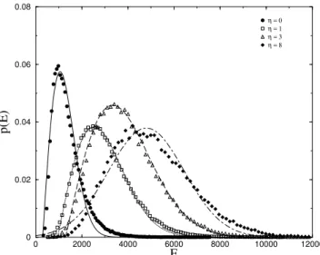
The distribution of the energies of the discrete config-urational states explored by the chain ofN = 48residues shown in Fig. 1, as it evolves under the above dynamics, is shown in Figs. 2, 3, for both positive and negativeη. Af-ter the first 5000 steps were discarded, the statistics were taken over 5000 steps of the trajectory. We checked that the statistics were stationary at this point so that we may safely assume that we have reached the attractor for this dynamics.
0 2000 4000 6000 8000 10000 12000 E
0 0.02 0.04 0.06 0.08
p(E)
η = 0 η = 1 η = 3 η = 8
Figure 2. The normalized energy histograms, averaged over10 ran-dom initial states for chains ofN = 48, for differentη≥0, along paths of104
steps, with the first5000steps discarded. The fits are to the Wigner distribution forη= 0,1,3and Gaussian distribution forη= 8.
The shape of the distribution essentially does not change
with η for η < 0, while for positive η the peak shifts
to successively higher values of the energy, and the distri-bution is distorted towards a Gaussian, indicating that the states explored are less correlated. These figures compare very favorably with the energy histograms obtained by Socci and Onuchic [40] for a Monte Carlo simulation on a lattice model of a proteinlike heteropolymer, the density of vibra-tional states found by ben-Avraham [6] and the ultraviolet
absorption spectra reported by Mach et al. [41]. It should be observed that the distributions which we obtain are also ex-tremely similar to the specific heat capacityCP as a function of temperature as found by Chan for different proteins. [42] It is interesting to note that it is also very similar to the distri-bution of Euclidean distances to the global energy minimum in the phase space of large atomic clusters [43].
0 1000 2000 3000 4000 5000 E
0 0.02 0.04 0.06 0.08 0.1
p(E)
η = −2 η = −4 η = −6
Figure 3. The normalized energy histograms, for chains ofN = 48, for differentη < 0(see Fig.2). The fits are to the Wigner distribution.
We were able to fit the simulation results very success-fully with a distribution of the Wigner form (Figs. 2,3)
fW(E) =a(E−E0)e−b(E−E0)
2
, (9)
forη=−6toη= 3. HereE0corresponds to the offset due to the lowest energy state attained for the differentη, and it can be seen that it shifts the distribution to higher values of the energy for higher values ofη. The distributions become Gaussian forη= 6andη= 8. (See Ref.[3], Table Ia,b for the values of the fitting parameters)
It should be mentioned that the same energy distribu-tions may be fit equally well (or better near the point E0 and in the far tail) by the “inverse Gaussian” [44], where the probability density is given by,
fIG(E) =
r A
2πE3 exp
·
−A(E−B)
2
2B2E
¸
. (10)
This has the same functional form as the distribution of first passage times over a distancedfor an Ornstein Uhlenbeck process [13, 14] with diffusion coefficientDand initial drift velocityv, in the regime of small times, if one makes the further identificationsA=d2/(2D)andB=d/v. The pa-rameters and estimated errors for the fits to the papa-rameters
A andB are given in Table II of Ref. [3]. Both the “dif-fusion constant” (mobility) and the “drift velocity” of the phase point along its trajectory in phase space depend on
C. Universality of the energy historgrams and the Ornstein-Uhlenbeck process
An Ornstein-Uhlenbeck (OU) process describes the dif-fusive motion of a particle subject to a drift velocity pro-portional to the distance from the origin [13, 14]. Such a process for a single particle in one dimension would be de-scribed by the Langevin equation,
dx dt =−
1
ζgx+ξ(t) (11) with a Hookean forceF(x) =−gxand a delta correlated random force ξ(t), h(ξ(t))2i = σ2. In the absence of the stochastic term which gives rise to diffusive motion, the ve-locity is simply proportional to the distance from the origin (or the point of equilibrium). For an initial displacement x(0) = d, the solution for the distribution of first passage times through the origin is given by
f(t) = 2yd
π1/2σ
µ ρ
1−y2 ¶3/2
e− ρy2d2
σ2 (1−y2) , (12)
whereρ=g/ζandy= exp(−ρt).
We would now like to show that both the Wigner distri-bution (9) and the inverse Gaussian distridistri-bution (10) arise as limiting forms in an OU process. Clearly, without the stochastic term, the solution for (11) is simply x =
dexp(−ρt) =dy. We see that (12) goes over, in the limit of large times, i.e.y ≪1, to
fW=
µ2ρ3/2 π1/2σ
¶ yde−ρd
2y2
σ2 . (13)
On the other hand, for very small times, (12) becomes, to leading order,
fIG= 2πdσ
2
(2πσ2t)3/2e
−(d−vt)2
2σ2t (14)
where we have definedρd=v.
Sincex= dyis the “distance remaining to the origin,” the distribution function (13) may just as well be consid-ered as a function of x. For late times, we getfW(x) ∝ xexp(−ρx2/σ2)which is in the form of the Wigner surmise (1). On the other hand, for very small times,x∼d(1−ρt) =
d−vt. The distance from the initial point,x˜ ≡(d−x)/v, becomes simply proportional to the time elapsed and we get the “inverse Gaussian”(10) form,
fIG(˜x)∼
µ λ
(2π˜x)3 ¶
e−λ2( ˜
x−µ)2
µ2 ˜x2
(15)
whereλ= (d/σ)2andµ= 1/ρ. It should be noted that (13 and 14) are numerically very similar.
Now let us observe that the energy E given in Eq.(2) obeys a one dimensional OU proces (11) under the dynam-ics given by (7). Since there is no explicit time dependence ofE, we have
dE dt =
X
i ∂E ∂ri ·
∂ri
∂t . (16)
Substituting from (7) we get,
dE dt =−
1
ζr X
i µ∂E
∂ri
¶2
+X
i ∂E
∂ri ·ξi(t) . (17)
From (2) we find
X
i µ
∂E ∂ri
¶2
= N E
ζr
+X
i,j,k i6=k
cikcjk(ri−rk)·(rj−rk) . (18) We see that the second term is like an average of the product of differences(ri−rk)·(rj−rk)over(i, j)pairs(i6=j),
and for a reasonably isotropic configuration, it vanishes. To the same approximation, we may assume that the second term in Eq.(17) is itself equal to a Gaussian stochastic noise, i.e., setξE(t) =KPijcij(ri−rj)·ξi(t) .This yields the required result, namely,
dE dt =−
N E ζr +ξE .
(19)
If under the given dynamics, theE distribution obeys one of the limiting forms (13) or (14), then the first passage time distribution for the attainment of the lowest energy state must obey, in turn, Eq. (12). This is the reason why the dis-tributions of first passage times for rather general global op-timization problems with quadratic cost functions [44] is the same as the form of the distribution of energy states which we find from our simulations.
That the same form is found experimentally for the spectral fluctuations of rather diverse confined systems of sufficient complexity [17, 16, 43, 45] seems to indicate that quadratic cost functions seem to be a sort of attrac-tor, under coarse graining, for a large space of many-body interactions. The seemingly universal behaviour which ben-Avraham finds for the density of vibrational states [6] and the ultraviolet absorption spectra reported by Mach et al. [41] for various proteins, also display very similar curves. Thus there seems to be a striking universality [8] not only between different protein-like structures, but also between different ranges of length and energy scales. It is actually surprising that the density of vibrational states should have a behaviour similar to energy histograms obtained under our dynamics, since the former involve inertial degrees of free-dom, while the latter arise from dissipative dynamics
It is also intriguing to compare the results for η ≥ 0
the energies of large atomic clusters, with successively fur-ther right-shifted peaks corresponding to distributions about higher metastable states.
D. Relaxation Behaviour
In order to investigate how the present model relaxes to equilibrium at a given temperature T, we have employed Metropolis Monte Carlo dynamics [20]. This consists of
a)choosing a pair(i, i′)of dihedral angles randomly on
the chain, and updating the (φi,φi′) in a way that preserves angular momentum, incrementing them in opposite direc-tions by∆φ=±2π/3,
b)accepting the move with unit probability if∆E ≤0
and with probabilityp= exp(−β∆E))for∆E >0, where β is an effective inverse temperature, β = (kBT)−1 with kBbeing the Bolzmann constant.
c)repeating the second step once before discarding the pair altogether and going to the first step.
0 2 4 6 8 10
lnt −3
−2 −1 0 1 2 3
ln(−ln(
ε)) 0 2 4 6 8 10
lnt
−14 −10 −6 −2 2
ln(
ε
)
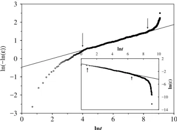
Figure 4. The decay with time (in Monte Carlo steps) of the energy, in arbitrary units, of anN= 100chain, along a Metropolis Trajec-tory of 104
steps, averaged over 20 runs. The initial configuration is random. The inverse temperature isβ = 0.3. The initial stage (inset) is fit by a power lawǫ(t)∼t−σwithσ= 0.49±0.01, and the late stage to a stretched exponential withα= 0.234±0.03.
We monitor the relaxation of the total energy as a func-tion of “time” measured in the number of MC steps, (i.e., the number of pairs (i, i′) sampled) until a steady state is reached, typically in about 10,000 steps for chains of N = 100. The results averaged over 20 randomly cho-sen initial configurations at zero temperature (β =∞) are shown in Fig. 4. Definingǫ ≡ (E −E0)/EI, whereE0 is the (time- averaged) equilibrium energy andEI, the ini-tial value, we find that it obeys a power law,ǫ(t)∼t−σwith σ= 0.49±0.01for the initial stages of the decay, while later stages can be fitted by a stretched exponentialǫ(t)∼e−tα withα= 0.234±0.003.
We also performed simulations for different values ofβ, for chains ofN= 48, averaging over 100 runs with random initial configurations. Forβ → ∞,β = 0.5andβ = 0.3, the above relaxation behaviour continues to hold and the ex-ponents do not seem to depend on β, with α ≃ 1/4 and σ≃1/2as given in Table I.
Table I: The exponentsσandαfound for the power law and stretched exponential decay of the total energy with time, for different chain lengthsN and inverse temperaturesβ. The fits were obtained from a weighted least-squares computa-tion.
N β σ ∆σ α ∆α
48 ∞ 0.57 0.01 0.281 0.004
0.5 0.56 0.01 0.30 0.04
0.3 0.57 0.01 0.25 0.03
100 ∞ 0.49 0.01 0.234 0.003
Clearly one may writeE(t), averaged over many inde-pendent runs, ashE(t)i = hE(0)−PM
i=1∆EiΘ(t−ti)i whereΘis the Heavyside step function andti =Pik−=01τk, withτkbeing the waiting time at thekth step, not to be con-fused with the symbol for the torques in subsection IIA. Tak-ing the time derivative one gets,
hE˙(t)i=h− M X
i=1
∆Eiδ(t− i−1 X
k=0
τk)i . (20)
At zero temperature, the expectation value ofE˙(t)can be calculated by carrying out an integration over the disti-bution of waiting times{τk}, and the distribution of energy steps encountered along the relaxation path. The expecta-tion value,hE˙(t)iis then,
hE˙(t)i=−h M X
j=1
∆Ejδ(t− i−1 X
k=0
τk)i∆E,τ . (21)
It is important to note that the distribution of waiting timesτkis dependent only on the configuration of the chain at the k’ th step and independent of the previous waiting times. Since the dynamics is just changing a pair of dihedral angles in opposite directions, for each conformation{φi} one may define an associated chain ofN(N −1)/2 sites, with each site corresponding to a pair of angles(i, i′)on the original chain. On the associated chain, a site will be as-signed the value 1 if the corresponding pair of angles has at least one “allowed” move, and the value 0 if both moves are “blocked” under the Metropolis dynamics at zero tem-perature. Now the probabilities of encountering allowed or blocked moves as one takes successive Monte Carlo steps are simply given by the density of 1’ s or 0’ s on the as-sociated chain at thekth relaxation step. Let us label these probabilitiespk andqk = 1−pk. Then, in thek’th confor-mation, the probability of making a transition after precisely τkblocked moves simply obeys the first passage time distri-bution [13],
(21) immediately, and we end up with a simple linear de-cay forE(t). By contrast, to see how the relaxation times depend on the state of the system, we may argue that the larger the energy loss in a relaxation event, the longer it will take for the phase point to make a transition out of this state. Sinceµkis roughly the expectation forτk, we assume that µk ∼ 1/∆Ek. With the assumption that the energy steps encountered along a relaxation path are independently distributed, i.e.,P(∆E1. . .∆EM) =QMs=1P(∆Es)for a process ofM steps, one finds,
hE˙(t)i=− 1
2π M X
j=1 h∆Eji
j−1 X
ℓ=1
Ijℓ(t) , (23)
whereIj,ℓ(t)is
Ij,ℓ(t) ≡ Z ∞
0
d(∆Eℓ)e− t
∆EℓP(∆Eℓ)
×
j−1 Y
k=0
k6=ℓ ¿
∆Eℓ
∆Eℓ−∆Ek À
∆Ek
. (24)
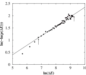
This is obtained by taking the integral representation for the delta-function in Eq.(21), and then performing the integrals over the τk with the probability distribution (22), and fi-nally performing the remaining integral using the residue theorem. Meanwhile we find that the probability distribu-tion of the energy differences encountered along a relaxadistribu-tion path, P(∆Eℓ), also is a stretched exponentialP(∆Eℓ) = Poexp(−(∆Eℓ)a), witha= 0.39±0.02(see Fig. 5). The angular brackets then take the form
∆Eℓ Z ∞
0
(∆Eℓ−∆Ek)−1exp(−(∆Ek)a)d∆Ek (25)
which we approximate by ∆Eℓexp(−(∆Ek)a). The in-tegration in equation (24) is then straightforward, leading, upon substitution in (23), to
E(t)∼t M X
j=1 µj−1
j ¶
exp(−ajtα) (26)
whereaj=j(1−a)(aj)−α(1 +α)−1and
α= a
a+ 1 . (27)
Substituting the above value ofawe getα= 0.28±0.01
which is the result we obtained from the fits to the MC sim-ulations within our error bounds.
5 6 7 8 9 10
ln(∆E)
0 0.5 1 1.5 2 2.5
ln(−ln(
p
(
∆
E
)))
Figure 5. The distribution of energy differences encountered along the relaxation path are fit to a stretched exponential. Level spacing histograms were formed for chains of N=48 and averaged over 100 runs for the zero-temperature Metropolis relaxation. The exponent aof the stretched exponential is found to be0.39±0.03.
The distribution of ∆E along a trajectory of the η– dynamics [3] is quantitatively different from the distribution of∆Eencountered along a Metropolis Monte Carlo path, and depends onη. This arises from the highly complex na-ture of the energy landscape, and the extremely important correlations that arise between the energy steps encountered depending upon how the phase space is being sampled. In particular, we have found out that in the limit of extremely largeη, where no cooperativity remains, the distribution of
∆Ealong a trajectory of the dynamics is Poissonian, which would have led toα= 1/2instead of1/4.
The relaxation to the native states for several real pro-teins was investigated by Erman [23, 24], who also finds a stretched exponential relaxation with α = 1/4. Ex-periments on real proteins and polymers [4, 21, 22] yield
0.2 ≤ α ≤ 0.4. Our results seem to be closer to 1/4 and smaller than the values most commonly found for pinned charge density waves [39], or spin-glasses [46], namely 1/3. It should also be noted that glassy behaviour is obtained here in the absence of quenched randomness, or of frustration arising from steric hindrances, which we do not take into account.
III
Hydrophobic chain near a h
y-drophobic boundary
In this section we will go back to the effective, entropy medi-ated hydrophobic interaction which is the driving force be-hind protein folding considered in the previous section as well as many other biological processes [4,5,47-50]. We will review some work which builds upon the model intro-duced by Widom and co-workers [26-30] to understand the microscopic mechanism leading to the effective attractive interaction between non-polar molecules placed in water, at least within a certain temperature interval. Then we will use this model to study the behaviour of a hydrophobic chain near a hydrophobic boundary, in two dimensions [25]. In trying to understand the behaviour of a hydrophobic chain in water, one must take into account both the hydrophobic interactions mediated by the orientational entropy of the wa-ter molecules, and the configurational entropy of the chain, while respecting its connectivity.
Although the behaviour of chains (or membranes) in the vicinity of spatial boundaries have been considered be-fore [51-53], these studies have concentrated on temperature independent interactions.
With the inclusion, to various degrees of accuracy, of the entropy of the chain, we are able to take into account the competition between the entropy of the water molecules which can be constrained by the presence of hydrophobic molecules in their neighborhood, and the entropy of the chain. We find that although at low and high temperatures, the chain prefers to be in a random configuration, detached from the wall, there is an intermediate temperature range where it is adsorbed on to the wall, at least for the relative values of the hydrogen bond, dipole-induced dipole and sol-vation energies which we have assumed.
The motivation behind studying this particular system is to shed light upon the chaperoning role which might be played by a hydrophobic surface in facilitating the folding process.
A. Decorated lattice model of hydrophobic interactions
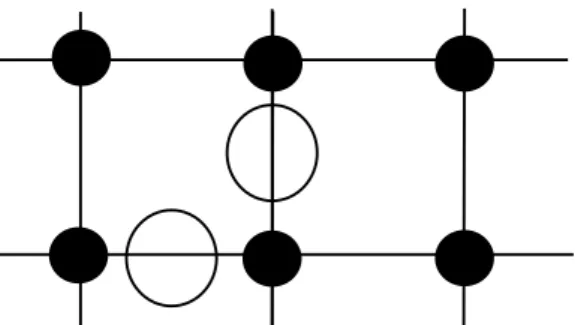
A decorated lattice model that mimics the solvent medi-ated hydrophobic interaction was suggested by Widom and his collaborators [26-30]. In this model,q-state Potts spins, {si}, are situated at lattice sites. These represent the polar solvent molecules. They can have any of theqdifferent po-larization directions. Hydrophobic molecules (HM), which are non-polar, can only be accommodated at interstitial sites, more precisely on the bonds connecting neighboring pairs (see Fig. 6). Lattice-gas variables,{σij}, σij = (0,1), lo-cated on the bonds(ij), indicate whether an interstitial site is empty or occupied by a HM.
Figure 6. Decorated lattice model. Lattice sites are occupied by water molecules (shown as filled circles); hydrophobic molecules (open circles) can only be accommodated at interstitial sites.
The interaction energy between a pair of solvent molecules is given by−δsi,1δsi+1,1(u−w)−u. The
occu-pation of the instertitial site is not allowed unless the neigh-boring pair of Potts spins are in the “special state” 1. The allowed states and their energies are summarized in Table II.
We have slightly modified this model, by introducing an energy of solvation and relaxing the prohibition against the occupation of the interstitial site in the disordered state. In this way we may actually write down a Hamiltonian for the water-and-hydrophobic solute system as,
HW =
X
<ij>
{δsi,sjδsi,1[σij(w−u) +u] +vσij¡1−δsi,sjδsi,1
¢
} . (28)
The interaction energies are ordered so that
w < u <0 < v , (29)
wherevmay be thought of as the solvation energy of the HM in the disordered state of the water molecules (see Table II). The ordering of the various interaction energies may be seen to follow from elementary considerations. The inter-action between water molecules and HM is always attrac-tive, because of the dipole-induced dipole interaction. On the other hand water molecules can form short lived tetrahe-dral structures [54, 55] stabilized by hydrogen bonds [56], i.e., a type of short ranged order. Because these structures have an open cage like space between them [57], a HM can be accommodated there without breaking any hydro-gen bonds. Thus, this “ordered” configuration is the min-imum energy configuration of water molecules in the pres-ence of a HM. In this model, the unique ordered state of the tetrahedrally bonded pentameric configurations of the wa-ter molecules [57], which is able to accommodate the HM without breaking any hydrogen bonds, is identified with the configuration where all thesiare in the state 1.
i.e., the zero level of the energy. When water molecules are randomly oriented, they can still have hydrogen bonds between them, though fewer in comparison to the ordered state. However, unlike the ordered state, there will be less open space between them. To be able to accommodate a HM in a disordered region of water molecules, further hydrogen bonds have to be broken. Thus, the insertion of a HM within this disordered phase of water molecules is energetically un-favorable.
The Hamiltonian Eq.(28) may be rewritten in terms of two-state variablesti, defined by
δsi,1 = ti. (30) withti = {1,0}, if we allow a temperature dependent “ex-ternal field.” In the partition function the multiplicity of the si 6= 1states can be taken care of by inserting a factor of
(q−1)for each Potts spin not in the ordered state, or a term −β(1−ti) ln(q−1)into the Hamiltonian, to get,
H =
N X
<ij>
{titj[σij(w−u−v) +u] +σijv}
−β−1 N X
i
(1−ti) ln(q−1) . (31)
Larger values ofqare more realistic sinceqis the num-ber of different orientations in which the solvent molecule can find itself. Apart from steric hindrances, we expect the orientation to be able to vary continuously, corresponding to some appropriateq → ∞limit [29]. Largerq values will clearly give rise to stronger entropy-mediated interactions between the solute molecules.
B. Effective hydrophobic pair interaction in the Mean Field Approximation
We would like to make use of this effective Hamiltonian to compute the self-interaction of a hydrophobic chain. To do this efficiently, we need an effective temperature depen-dent pair potential between the elements of the chain. In one dimension, one could perform a trace over the mediat-ing solvent molecule between two HM, to obtain an effective interaction. However, in two or higher dimensions, correla-tions between solvent molecules may be built up over many different paths. Therefore we decided to compute the effec-tive interactions between the solute molecules (without any effect felt from the presence of a wall) in the Mean Field Approximation. This is the subject of this section.
In the MFA, the Hamiltonian (31)on a cubic lattice ind dimensions, can be written as
HMF =
2d X
j=1
{thti[σj(w−u−v) +u] +σjv} −β−1µ(1−t) ln(q−1). (32) where the sum runs over the bonds pointing to the near-est neighbor sites. The field htiis the mean value of the
random variablestj associated with the neighboring water molecules, and it will be determined self-consistently. We have insertedµfor later convenience in computing expec-tation values, and will otherwise set it to unity. We ob-tain the effective pair interactions between the solute (HM) molecules by performing thetsum in the partition function.
The partition functionZis defined as Z= X
{σi},t
e−βHMF[t,{σi}] , (33)
i= 1, . . . ,2d, andhtimust be found from
1− hti = [ln(q−1)]−1 ∂
∂µlnZ|µ=1 (34) which we solved numerically for each given temperatureT, ford= 2.
We may define all the possible effectivep-body interac-tions that may be built from these lattice gas variables, by writing the effective Hamiltonian
Heff = −k0−k1X i
σi−k2 X
(ij) σiσj
− k3X (ijk)
σiσjσk−k4Πiσi , (35)
where (ij) denotes nn and nnn pairs and (ijk) triplets. Note that the nearest neighbor (nn) and next nearest neigh-bor (nnn) pairs are indistinguishable from each other in this “tree” approximation, since the bonds issuing from the sin-gle central site may be freely interchanged with one another. The interaction constants may be determined by setting
Z =X
{σi}
e−βHeff[{σi}] . (36)
By considering terms with all theσi set to zero, only one different from zero, or a pair of them different from zero, etc., one is able to determine all the coupling constantskp.
For the the two-body interactionsk2, which we will call M(β)from now on to simplify the notation, we find,
eβM(β) = e
−2β[hti(w−v+u)+v] + (q−1)e−2β v £
e−β[hti(w−v+3u)+v] + (q−1)e−β v¤2 ׳e−4β uhti+q−1´. (37)
0.0 0.5 1.0 1.5 2.0 2.5
β |u|
0.00 0.05 0.10 0.15
0.20 q = 15
q = 10 q = 5
β Μ
Figure 7. Effective, temperature dependent nn and nnn interaction energies between hydrophobic residues in water, in the MF approx-imation to the decorated lattice model [28]. Note thatM =k2 en-ters with a negative sign into the effective Hamiltonian in Eq.(35). Hereq is the number of different orientations which can be as-sumed by the water molecules. The effective interaction is stronger for largerq. The coupling constants for the decorated lattice model have been taken asw=−1.5, u=−1, v= 1.
To the lowest approximation [30] we will neglect the plaquette and triplet couplingsk4andk3as being of higher order in the fluctuations. The linear term we will also ne-glect, because it is like a chemical potential, and this will be taken into account in the wall-particle effective interaction which we will now calculate in a one-dimensional approxi-mation in the next subsection. The constant term of course cancels in all the expectation values, and may therefore be dropped from the start.
C. Effect of the boundary
In order to be able to estimate in closed form the effec-tive interaction of a HM with the hydrophobic boundary, we will consider a one dimensional system, and compute the ef-fective interaction between a hydrophobic insertion and the hydrophobic boundary from the free energy difference re-sulting from this insertion. We will then use this as an ap-proximation to the true interaction between the solute and the hydrophobic wall, in the unique normal direction to the wall (a linear boundary) in two dimensions.
The Hamiltonian in Eq.(31) becomes, in one dimension,
H =
N X
i
{titi+1[σi(w−u−v) +u] +σiv −β−1(1−ti) ln(q−1)} (38) ≡
N X
i
Hi[ti, ti+1, σi] .
ForNbeing the length of the one-dimensional lattice of water molecules, the free energy costF(N, T, r)of adding only one HM at an interstitial a distancerfrom the wall at temperatureT is given by
−βF(N, T, r) ≡ ln
µZ(N, T, r) Z0(N, T)
¶
, (39)
whereβ−1=k
BT as usual,Z0(N, T)is the partition func-tion of the one dimensional system withσi= 0for alli, that is, no HM molecules, andZ(N, T, r)is the partition func-tion computed in the presence of one HM a distancerfrom the wall. The effective interaction between the wall and a single HM is thus given by the free energy cost of bringing HM from bulk to distancerfrom the wall,
FN(I)(1, r) = F(N, T, r)− F(N, T, rb), (40) whererbmeans a displacement from the wall beyond which the effect of the wall is no longer perceptible, namely a bulk site. In the thermodynamic limit
F(I)(1, r) = lim
N→∞F
(I)
N (1, r). (41) To compute the partition functions in (39), we used the transfer matrix method. From Eq.(38), the transfer matrices in one dimension are obtained as
T(σi) =hti|e−βHi[ti,ti+1,σi]|ti+1i. (42) Thus, the transfer matrix is conditional on the presence (or absence) of an interstitial HM at each bond connecting two water molecules, and we find,
T(0) =
µ
e−β u (q−1)1 2
(q−1)12 (q−1)
¶
, (43)
T(1) =
µ
e−β w e−βv(q−1)1 2
e−β v(q−1)1
2 e−β v(q−1)
¶ ,(44) for the two possible resulting transfer matrices. To get the transfer matrices in a more symmetric form, we have rewritten the third term in the Hamiltonian (Eq.(38)) as −12β−1(2−t
i−ti+1) ln(q−1). ¿From Eq. (40), we get, with one HM inserted at a distancerfrom the wall,
−βFN(I)(1, r) = lnX
k
h1|Tr−1(0)T(1)T(0)N−r|ki −lnX
m
h1|TN−1(0)T(1)|mi. (45)
Notice that the left-most vector is fixed to be unity, sig-nalling the presence of the hydrophobic wall. In the ther-modynamic limitN → ∞, this reduces to,
−βF(I)(1, r) = lnX
ijk
AiTij(1)a1ja1k
−lnX
ij
a11a1jTji(1) , (46)
where we have defined
Ai≡a11a1i+ (λ2/λ1)r−1a21a2i , (47) with
λ1,2 ≡ 1
2e
−β u{1 + (q−1)eβ u ± £
being the eigenvalues of T(0), andakl the elements of its kth eigenvector.
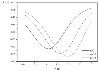
We will use F(I)(1, r), which we have calculated e x-actly in one dimension (Fig. 8), to give us an estimate of the interaction between the HM and the hydrophobic boundary in two dimensions.
Figure 8. The effective interaction potential of a residue with the hydrophobic wall for different values ofq, atr = 1, at differ-ent inverse temperatures. The interaction coefficidiffer-ents of the lattice model were chosen as in Fig. 7.
Hydrophobic chain with intra-chain and chain-boundary interactions
We are interested in the behavior of a hydrophobic poly-mer chain in the presence of a hydrophobic wall. This means we have to respect the connectivity of the chain in perform-ing the trace over the lattice gas variables correspondperform-ing to the HM. In other words, the phase space consists of allowed chain configurations.
To be able to treat the model at least in a semi-analytical way, we have considered two simplified sets of chain con-figurations, which we will outline below.
1. Modular chain or SOS model
We define a set of elementary modules, from which a large number of chain conformations can be built, such that only nearest neighbor modules come within the interaction range of each other. The subset of configurations that can be generated by random combinations of the modules that are shown in Fig. (9a) can clearly be seen as graphs (taking the boundary as the axis) without overhangs, as in a restricted solid-on-solid (SOS) model [58] in (1+1) dimensions, where successive steps are constrained to differ by at most one unit of height. Making use of the linearity of the chain and the restriction to nearest neighbor interactions between the mod-ules, we used the transfer matrixalong the chainto solve the partition function for our model Hamiltonian.
r
r
i
i
(1) (2) (3)
Figure 9. a) (Top panel) Elementary modules used to generate SOS like chain configurations which only allow nearest neighbor inter-actions between the modules, via nn or nnn interinter-actions between the hydrophobic residues. b) (Lower panel) Nearest and next near-est neighbor interactionsM(β)between HMs on the chain are in-dicated as wavy and dashed lines, respectively.
We labeled the modules in Fig. (9a) as1,2,3from left to right. A chain configuration is uniquely specified by as-sociating a variable, ui = {1,2,3},i = 1, . . . , Nm, with each module along the chain, and by specifying the distance of the first module from the wall. Note that the number of residues along the chain is given by2Nmin this case. The interaction energy of each residue with hydrophobic wall is computed using F(I)(1, r). We took M(β) defined in Eq.(37), to be the interaction energy between nearest and next nearest neighbor residues (see Fig.(9b)). Note that the nearest neighbor interaction (wavy line) connects residues belonging to modules twice removed from each other. Yet, since this occurs only in the(i, i+ 1) = (2,3)or (3,2) com-bination,independentlyof the identity of thei−1st module, it can still be accomodated within a nearest-neighbor Hamil-tonian.
We model the effective Hamiltonian of a polymer with
Nmmodules as,
Hc = −
Nm
X
i
{M(β)hui|Γ|ui+1i
+h1(ri−1, ri)}. (49)
The vectors|uii correspond to the three states of the vari-ableui, i.e.,(1,0,0),(0,1,0)etc., so that the coefficient of the pair interactionM(β)is conveniently written in terms of
Γ =
0 2 2
0 2 3
0 3 2
0 1 2 3
β |u|
1 2 3 4 5
v = 1 ( q = 10 ) v = 1 ( q = 5 ) v = 0.5 ( q = 5 )
<rcm>
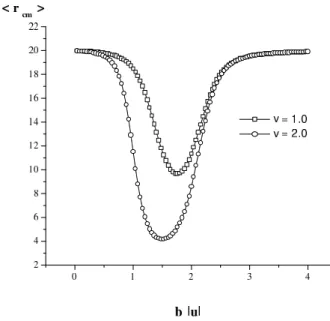
Figure 10. The average center of mass displacement from the boundary, of the hydrophobic chain with 60 residues in the SOS approximation, for different values of solvation energy,v, and dif-ferent values ofq. For computational purposes, the width of the channel was chosen to be 12 lattice spacings.
The second term is the free energy cost of adding HMs to the solvent matrix,h1(ri, ri−1) =−F(I)(1, ri−1)−F(I)(1, ri). The distance of the second residue on theith module from the wall,ri, is found fromri =r+ρi, whereris the dis-tance of the first module from the wall, and
ρi = i X
j=1 ¡
δuj,2 − δuj,3 ¢
. (51)
Note that the displacement of the first residue on the ith module is the same as that of the second residue on thei−1st module, and therefore the expression forh1follows.
The partition function of the polymer is, Z = X
r X
{u}
e−β Hc. (52)
Explicitly,
Z = X
{ri},{ui}
hr1, u1|U|r2, u2ihr2, u2|U|r3, u3i. . . . . .hrNm−1, uNm−1|U|rNm, uNmi. (53) Here,|ri, uiiareM×∋dimensional vectors, withMbeing the size of the system in the direction orthoganal to the wall. The transfer matrixU is given by a direct product
U =
3 X
ζ=1
W(ζ)⊗R(ζ) (54)
with
Wkℓ(1) = δℓ,1 (55)
Wkℓ(2) = δℓ,2£e2βM(δk,1+δk,2) +e3βMδk,3¤ (56)
W(3) = (2⇌3) , (57)
wherek, ℓ= 1,2,3,(2⇌3)indicates an interchange of the indices 2 and 3 in the previous equation, and
R(γηζ) = δζ,1δγ,ηe−2βF I(1,γ)
+ δζ,2δγ,η−1e−β[F
I(1,γ)+FI(1,η)]
+ δζ,3(γ⇌η) , (58)
whereγ, η = 1, . . .Mandζ = 1,2,3. We note that only the diagonal, upper diagonal and lower diagonal elements of the matricesR(ζ)are different from zero. However we have not been able to find a way to analytically diagonalize the matricesU, or, for that matterR; they are not simply cyclic, but the matrix elements depend directly on the row (or col-umn) index through the functionsF(I)(1, r
i). (See Eq.(13)). Therefore we have had to perform the matrix multiplications numerically.
We calculated the center of mass distance of the hy-drophobic polymer from the hyhy-drophobic boundary,
hrcmi = 1
Nm h
Nm X
i rii
= 1
Z
1
Nm Nm X
i=1 X
Ω
hr1u1|Ui|riuiiri hriui|UNm−i|rNmuNmi (59)
where the sum over the setΩshall henceforth mean a trace overr1, u1, ri, ui, rNm, uNm. Defining a3× Mvector,|φi such that
hφ|= (1 0 0 1 0 0 1 0 0. . . 1 0 0) (60)
one may slightly rewrite Eq.(59) as,
hrcmi = 1
Z
1
Nm Nm X
i=1 X
Ω
hr1u1|Ui|riuiihφ|riuii hriui|UNm−i|rNmuNmi . (61)
0.5 1.0 1.5 2.0 2.5 3.0 3.5
β |u|
39 43 47 51
v = 1 ( q = 10 ) v = 1 ( q = 5 ) v = 0.5 ( q = 5 )
<L>
Figure 11. Mean length of the hydrophobic chain with60residues, projected on to the boundary, in the SOS approximation. Different values of solvation energy,v, and different values ofqare shown for comparison.
Asβ→0(high temperatures) the intrachain interaction
M also goes to zero, the entropy of the chain becomes the
determining factor, and the chain floats free. At low
tem-peratures, as the entropy term in the free energy becomes negligible, the equilibrium state is determined by energetic considerations, and the polymers desorb and take on ran-dom configurations, constraining a large number of water molecules in their neighborhood.
The average end to end distance of the polymer chain, projected on to the boundary, is given by
hLi=Nm+
*Nm X
i
δui,1
+
. (62)
Defining|ψiby,
hψ|= (1 0 0 2 0 0. . . 1
3(k+ 2) 0 0. . .M0 0) , (63) we get,
hLi=Nm + 1
Z
1
Nm
Nm
X
i=1
X
Ω
hr1u1|Ui|riuiihψ|riuii
hriui|UNm−i|rNmuNmi. (64)
The temperature dependence is reported in Fig. (11). In the limitβ→0, clearlyhLi=Nm(1 +13), which is what one sees in Fig.(11), with Nm = 30. It is interesting to note the non-monotonic behaviour ofhLiwithin the region of in-terest, namely the temperature interval for which the center of mass lies very close to the wall. This non-monotonicity arises from the competition between the entropy mediated effective self-interaction of the chain (leading to smallerL) and the interaction with the wall (completely shielding one side from the water by stretching out to adsorb on to the wall). This behaviour is also observed in the models we have considered in the subsequent sections.
Although the SOS model is exactly solvable in princi-ple, it is unable to take into account configurations of the
chain which fold on themselves, and we therefore have also considered a model where such conformations are allowed.
2. Then-fold model
In this section we take a different subset of chain con-figurations over which to perform exact summations. These configurations are shown in Fig.(12). If the length of the polymer is Nl then the energy of a chain with an integer number of foldsNl/n, is given by
Hn =
Nl
n
n
X
i=1
F(I)(1, r+i−1) −M νn(1−δn1−δnNl) (65) where r is the distance from the wall and νn = 3(n− 1)(Nl/n−1) is the total number of nearest neighbor and next nearest neighbor pairs in this configuration. The parti-tion funcparti-tion
Z=X
r
′ X
n
e−βHn (66)
is nontrivial to sum, again because of the complicated way in which the functionsF(I)(1, r+i−1)depend on their arguments, viz. Eqs.(46,47), and the nonlinear dependence ofνnonn.
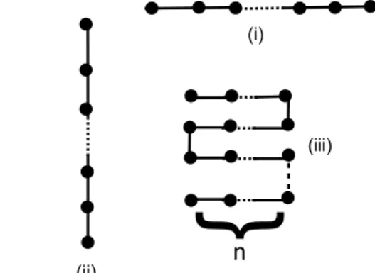
(i)
(ii)
(iii)
{
n
Figure 12. Polymer configurations included in the exact enumera-tion of then-fold model.
The center of mass displacement from the wall can be obtained in principle from
hrcmi=Z−1
X
r
′ X
e−βHn[r+1
2(n−mod2n)] , (67) where the prime indicates that the summation is only over exact divisors ofNl. The mean value of the vertical distance between the first and last monomer ishLi=hNl/ni, which can be calculated from,
hNl/ni =
1
Z X
r ′
X
n
Nl
n e
−β Hn. (68)
To obtain these quantities, the partition function and the expectation values were summed numerically, insert-ing, for each different value ofβ, the numerical value of
course a finite set of values had to be chosen forr. The re-sults we find are qulitatively and quantitatively very close to our earlier results for the SOS-like model. [25]
In the low temperature limit, increasing the number of HM-water nn pairs lowers the energy and this is favorable since the entropy term in the free energy is suppressed, and the chain takes on relatively open, random configurations. At intermediate temperatures where the hydrophobic inter-actions are the most effective, the chain prefers to neigh-bor the hydrophobic wall at as many nn sites as possible, and therefore is adsorbed on the wall in the unfolded state. As the temperature is raised somewhat more, effective self interactions of the chain become more important, and the chain is in a more folded state, although still adhering close to the wall. At high temperatures it is advantageous to mini-mize the number of nearest neighbor sites at which the chain is in contact with water molecules, since the entropy of the water molecules is rather large, especially for largeq. On the other hand, the entropy of the chain also favors open configurations, which win out in the high temperature limit. We found, withNl = 50,hLiis close toNl3/4 = 18.8, at both extremes, with the power being that of the self avoiding walk in two dimensions.
E. Monte Carlo simulations
Monte Carlo computations for 3×10⁵ random self avoiding walk configurations of length N = 20 were reported in Ref. [25]. Here we will report the results from 3×10⁴ configurations , generated via a genetic algo-rithm [60]. If a random walk passes through any lattice point which it has already visited, the configuration is dis-carded, and a new one generated. Each successfully gen-erated configuration was decorated with the interaction po-tentials F(I)(1, r) andM(β)from Eqs.(40,37), to finally compute the expectation values for the center of mass dis-placement from the wall and the longitudinal component of the end to end distance, in the canonical ensemble. The re-sults we find (Figs. 13,14) are surprisingly close to those shown in Figs. (10,11), to then-fold model results and to the MC results in [25].
IV
Thermodynamics of early protein
function
It has long been appreciated [34] that proteins are unique among possible amino acid chains in being able to fold into a unique “native state” and reversibly unfold to a random coil. Synthetically produced amino acid chains have degenerate ground states. Moreover, small to medium sized proteins typically fold and unfold at one go, without any intermedi-ary states between the folded and the unfolded ones. This can be quantified by various measures of so called “two-state cooperativity”[42, 61]. It is a challenge to understand the mechanism by which such amino-acid sequences were selected in the course of evolution or how biological evolu-tion as we know it came to being in the first place. It would seem
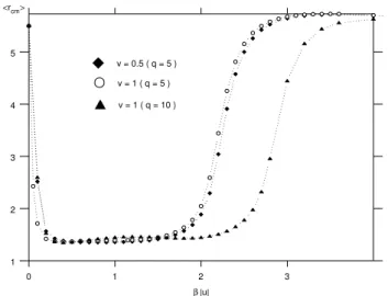
Figure 13. Monte Carlo results (see text) for the average center of mass displacement from the wall, of a polymer with20residues, for different values of the solvation energy,v, and forq = 10, u=−1.0, w=−1.5, on a 40×40 lattice. The longitudinal axis is the inverse temperature in units ofkB/u.
Figure 14. The average longitudinal component of the length of the hydrophobic polymer, for the same parameters as in the previous figure.
to be self-evident that the highly specific functions dis-charged by proteinsin vivowould not have come into play unless two-state cooperativity had already been selected via some pre-biotic mechanisms. In Ref. [32], we have argued for a basic thermodynamic function which could have been fulfilled by proteins, namely that of a refrigerant in an ad-sorption refrigeration process.
ran-dom jumble and transforming them into an ordered chain. As a result, the information carried by RNA is translated into specificintra-chain interactions as well as interactions with the ambient water, subject to given boundary condi-tions. Once the peptide chain is formed and wiggles free from the RNA molecule, it can behave as an active Brown-ian particle [63] responding to variations in temperature or other external stimuli in specific ways which enable it, in turn, to act upon them.
A common assumption regarding compartition is that porous rock could have played host to prebiotic pro-cesses. [2, 64] Recent evidence has been providedby Mar-tin and Russel [65] that life could have originated in iron monosulfide precipitates on the ocean floor, whose pores, lined with certain lipids, may have provided the first simple cell-like structures.
We have already shown that due to hydrophobic interactions[25] those peptide chains that are near hydropho-bic surfaces may adsorb on such surfaces at least within given temperature intervals. It may be conjectured that rock surfaces, with some lipids present, are favorable sites for adsorption, and act as guides for the peptide chains, helping them to fold. Upon folding, as a result of the reduction in entropy, heat will be given off, mostly to the surface of the rock. For special sequences, with specific intra-chain inter-actions, this folded state will be stable. If, now, the surface on which the proteins have adsorbed is heated, say by the emission of a hydrothermal vent [65], the chain will detach itself from the rock surface. If it is carried along by convec-tive currents away from the heated wall, and in particular towards a cooler pocket, where, say it encounters a region of with a high pH, which lowers the denaturation temper-ature, this is where it will unfold, absorbing heat from its surroundings.
This, in fact describes an adsorption-refrigeration cy-cle driven by low quality heat [66-71]. The efficiency of such a refrigeration cycle operated by proteins undergoing a folding-denaturation transition would depend strongly on two parameters: the entropy gap between the folded and un-folded states of the amino-acid chain, and the rate of the folding-unfolding transition. One may now hypothesize that the accidental establishment of such a refrigeration cycle provided an evolutionary advantage to those RNA molecules that coded proteins that were efficient coolants, since, in an overheated environment, lower temperatures could enhance the replication rates of RNA. This completes the hypercycle. If this scenario is correct, the fates of RNA chains would from then on be bound with the synthesis- and eventual evolution- of polypeptides. Those RNA sequences would be selected for, that were able to synthesize proteins that folded into lower entropy states, and did this in a very short time. Present day biological proteins have unique ground states leading to large entropy gaps. Small single domain proteins fold into their secondary structures within milliseconds [72], or even faster [73].
What we would like to emphasize here is the point of view that simple chemical and physical processes which set
the stage for biological evolution, must already have pro-vided a great deal of variety and complexity upon which the fortuitous emergence of self-replicating entities posessing a hereditary code could elaborate.
Acknowledgements
AE gratefully acknowledges partial support from the Turkish Academy of Sciences.
References
[1] M. Eigen, Naturwissenschaften,10, 58 (1971).
[2] J. M. Smith and E. Szathm´ary,Origins of Life(Oxford Uni-versity Press, Oxford, 1999).
[3] E. T¨uzel, A. Erzan, J. Stat. Phys.100, 405 (2000).
[4] H. Frauenfelder, S. G. Sligar, P. G. Wolynes, Science,254, 1598 (1991).
[5] P.G. Wolynes, J.N. Onuchic, and D.Thirumalai, Science276, 1619 (1995)
[6] D. ben-Avraham, Phys. Rev. B47, 14559 (1993).
[7] K.A. Dill, S. Bromberg, K. Yue, K.M. Feibig, D.P. Yee, P.D. Thomas, and H.S. Chan, Protein Science4, 561 (1995).
[8] M.M. Tirion, Phys. Rev. Lett.77, 1905 (1996).
[9] T. Haliloglu, I. Bahar, and B. Erman, Phys. Rev. Lett. 79, 3090 (1997).
[10] B. Erman and K. Dill, J.Chem. Phys.112, 1050 (2000).
[11] B. Erman, Comp. Theor. Polym, Sci.9295 (1999).
[12] B. Ewen, D. Richter, in Elastomeric Polymer Networks, edited by J. E. Mark and B. Erman, (Prentice Hall, 1992) p. 220.
[13] W. Feller,An Introduction to Probability Theory and its Ap-plicationsVol. II (Wiley, New York, 1957), p. 332ff.
[14] H. Risken, The Fokker-Planck Equation (Springer, Berlin, 1984).
[15] E. Wigner, Proc. Cambridge Phil Soc.47, 790 (1951); Ann. Math.62, 548 (1955).
[16] T. Brody, J, Flores, J.B. French, P.A. Mello, A. Pandey, and S.S.S. Wong, Rev. Mod. Phys.53, 385 (1981).
[17] C.E. Porter, Statistical Theories of Spectra: Fluctuations
(Academic Press, New York, 1965).
[18] C.E. Porter, J. Math. Phys.4, 1039 (1963).
[19] M.L. Mehta,Random Matrices and the Statistical Theory of Energy Levels(Academic Press, New York 1967).
[20] E. T¨uzel, A. Erzan, Phys. Rev. E61, 1040 (2000).
[21] J.L. Green, J. Fan, and C.A. Angell, J. Phys. Chem.98, 13780 (1994).
[22] J. Colmenero, A. Arbe, and A. Algeria, Phys. Rev. Lett.71, 2603 (1993).
[23] B. Erman, I. Bahar, Macromol. Symp.133, 33 (1998).
[24] I. Bahar, B. Erman, F. Kremer, and E.W. Fischer, Macro-molecules,25, 816 (1992).
[26] A.B. Kolomeisky, B. Widom, Faraday Discuss.112, 81-89 (1999).
[27] B. Widom, Pol. J. Chem.75, 507 (2001).
[28] G.T. Barkema and B. Widom, J. Chem. Phys. 113, 2349 (2000).
[29] G.M. Sch¨utz, I. Ispolatov, G.T. Barkema, and B. Widom, Physica A291, 24 (2001).
[30] D. Bedeaux, G.J.M. Koper, S. Ispolatov, and B. Widom, Physica A291, 39 (2001).
[31] B. Widom, P. Bhimalapuram, and K. Koga, “The Hydropho-bic Effect,” (review article), to appear in Phys. Chem and Chem. Phys. (2003).
[32] E. T¨uzel, A. Erzan, “A Thermodynamic Model for Prebi-otic Protein Function,” cond-mat/0107315, and submitted for publication in Phys. Rev. E.
[33] A. Yu. Grosberg, J. Stat. Phys.38, 149 (1985).
[34] P.J. Flory,Statistical Mechanics of Chain Molecules, (Inter-science, N.Y., 1969).
[35] T. Halpin Healy and Y.C. Zhang,Physics Reports,254, 215 (1995).
[36] J. Krug, P. Meakin, and T. Halpin-Healy, Phys. Rev. A45, 638 (1992).
[37] A. Erzan, E. Veermans, R. Heijungs, and L. Pietronero, Phys. Rev. B41, 11522 (1990).
[38] E. Veermans, A. Erzan, R. Heijungs, and L. Pietronero, Phys-ica A166, 447 (1990).
[39] G. Parisi and L. Pietronero, Physica A179, 16 (1991).
[40] N. D. Socci, J.N. Onuchic, J. Chem. Phys.103, 4732 (1995).
[41] H. Mach, D.B. Volkin, C.J. Burke, and C.R. Middaugh, “Ultraviolet Absorption Spectroscopy,” in B.A. Shirley ed.,
Methods in Molecular Biology,edited by B.A. Shirley, Vol. 40: Protein Stability and Folding (Humana Press, Totowa, New Jersey, 1995) p. 91.
[42] H.S. Chan, Proteins: Structure, Fucntion and Genetics,40, 543 (2000).
[43] M.A. Miller, J.P.K. Doye, and D. Wales, Phys. Rev. E60, 3701 (1999).
[44] C.N. Chen, C.I. Chou, C.R. Hwang, J. Kang, T.K. Lee, and S.P. Li, Phys. Rev. E60, 2388 (1999).
[45] D. Bohigas, M. J. Giannoni, and C. Schmidt, Phys. Rev. Lett. 52, 1 (1984).
[46] M. Mezard, G. Parisi, and M. A. Virasoro,Spin Glass Theory and Beyond(World Scientific, Singapore, 1987).
[47] A. Ben-Naim,Hydrophobic Interactions(Plenum, New York and London, 1980).
[48] A. Ben-Naim, J. Chem. Phys.90(12), 7412 (1989).
[49] A. Sali, E. Shakhnovich, J. Mol. Biol.235, 1614 (1994).
[50] K.A. Dillet al., Protein Science,4, 561-602 (1995).
[51] R.R. Netz, D. Andelman, Oxide Surfaces(Marcel Dekker Inc., New York, 2000)
[52] A. Stella, T. Jr. Phys.,18, 224 (1994).
[53] E. Eisenriegler, Polymers near surfaces (World Scientific, Singapore, 1993).
[54] G. N´emethy, H.A. Scheraga, J. Chem. Phys.,36, 3382 (1961)
[55] R.A. Horne ed.,Water and Aqueus Solutions Structure, Ther-modynamics, and Transport Processes(John Wiley & Sons, London, 1972)
[56] C. Kittel,Introduction to Solid State Physics(John Wiley & Sons,Inc., 1986)
[57] M. Canpolat, F.W. Starr, A. Scala, M.R. Sadr-Lahijany, O. Mishima, S. Havlin, and H.E. Stanley, Chem. Phys. Lett. 294, 9 (1998); H.E. Stanley, S.V. Buldyrev, M. Canpolat, O. Mishima, and M.R. Sadr-Lahijany, Physica A257, 213 (1998) and Phys. Chem. Chem. Phys.2, 1551 (2000).
[58] G.H. Gilmer and P. Bannema, J. Appl. Phys.43, 1347 (1972); H. van Beijeren, Phys. Rev. Lett.38, 993 (1977); for a review see D.B. Abraham, inPhase Transitions and Critical Phe-nomena, Vol. 10, edited by C. Domb and J. Lebowitz, (Aca-demic Press, New York, 1986).
[59] J.D. Bryngelson, E.M. Billings, Physics of Biological Sys-tems(Springer, Berlin, 1997)
[60] Y. S¸eng¨un, Diploma Thesis, ITU (2003).
[61] H. Kaya and H.S. Chan, Phys. Rev. Lett.85, 4823 (2000).
[62] M. Eigen, Steps towards Life, a Perspective on Evolution
(Oxford University Press, Oxford, 1992); also see M. Eigen and P. Schuster, The Hypercycle (Springer, Berlin, 1979) p.109.
[63] F. Schweitzer, “Active Brownian Particles with Internal En-ergy Depot” in Traffic and Granular Flow ’99: Social, Traffic and Granular Dynamics, edited by D. Helbing, H.J. Herrmann, M. Schreckenberg. D.E. Wolf, (Springer, Berlin, 2000) p. 161; U. Erdmann (a), W. Ebeling, L. Schimansky-Geier, and F. Schweitzer, Eur. Phys. J. B15, 105 (2000).
[64] S.A. Kauffmann, The Origins of Order: Self–Organization and Selection in Evolution(Oxford University Press, Oxford, 1999).
[65] W. Martin, M.J. Russell, Phil Trans. Royal Soc. B (Biol. Sci.) (London),358, 59 (2003).
[66] Y.A. C¸ engel and M.A. Boles, Thermodynamics: an Engi-neering Approach (McGraw Hill, N.Y., 1996; in Turkish translation by Literat¨ur Yayınevi, Istanbul, 1996) p. 549.
[67] J.S. Hsieh,Solar Energy Engineering(Prentice Hall, Engle-wood Cliffs, New Jersey, 1986) p.303.
[68] Y. Teng, R.Z. Wang, and J.Y. Wu, App. Therm. Eng.17, 327 (1997).
[69] F. Meunier, F. Poyelle, and M.D. LeVan, App. Therm. Eng. 17, 43 (1997).
[70] M. Pons, App. Therm. Eng.17, 615 (1997).
[71] H.T. Chua, K.C. Ng, A. Malek, and N.M. Ono, J. Appl. Phys. 89, 5151 (2001).
[72] A. Fersht, Structure and mechanism in protein science: a guide to enzyme catalysis and protein folding(W. H. Free-man, New York, 1998).
![Figure 7. Effective, temperature dependent nn and nnn interaction energies between hydrophobic residues in water, in the MF approx-imation to the decorated lattice model [28]](https://thumb-eu.123doks.com/thumbv2/123dok_br/18979909.456656/10.892.122.427.115.348/effective-temperature-dependent-interaction-energies-hydrophobic-residues-decorated.webp)