Article
Printed in Brazil - ©2017 Sociedade Brasileira de Química 0103 - 5053 $6.00+0.00
*e-mail: [email protected]
Comparison of ICP OES and LIBS Analysis of Medicinal Herbs Rich in Flavonoids
from Eastern Europe
Daniel F. Andrade,a Edenir Rodrigues Pereira-Filho*,a and Pawel Konieczynskib
aGrupo de Análise Instrumental Aplicada (GAIA), Departamento de Química (DQ),
Centro de Ciências Exatas e de Tecnologia (CCET), Universidade Federal de São Carlos (UFSCar), P.O. Box 676, 13565-905 São Carlos-SP, Brazil
bDepartment of Analytical Chemistry, Medical University of Gdansk, Gen. J. Hallera 107,
80-416 Gdansk, Poland
Essential and toxic metals were determined in eighteen samples of medicinal herbs from Poland, Lithuania and Serbia by means of laser-induced breakdown spectroscopy (LIBS) and inductively coupled plasma optical emission spectrometry (ICP OES). Calcium, K and Mg concentrations were obtained in % (m/m) and other metals (Na, Co, Cu, Fe, Mn, Ni, Zn, Cd, Cr and Pb) in mg kg-1. The fact that the herb samples analyzed belonged to specific plant species and represented
different morphological plant parts explained the characteristic distribution in two-dimensional scores plots obtained by principal component analysis (PCA). A strong correlation of LIBS results was achieved in comparison to those obtained by ICP OES for Ca, K and Mg. Differences in the types of infusions were observed, in that leaves are related to Zn and Ni concentrations, leaves and flowers to Co, Ca and Mn concentrations and flowers to K, Na, Mg and Fe content.
Keywords: medicinal herbs, essential and toxic metals, LIBS, ICP OES, chemometrics
Introduction
Quantitative analysis of essential and toxic metals present in medicinal herbs is an important issue for researchers worldwide. Its significance is illustrated by the numerous studies to determine the levels of metallic and non-metallic elements, macro- and microelements, essential and toxic elements in plants used medicinally, which have employed a myriad of instrumental analytical techniques. The list includes several spectroscopic methods, for instance, atomic absorption spectrometry (AAS),1,2 and related techniques such as inductively coupled plasma optical emission spectrometry (ICP OES)3,4 and inductively coupled plasma-mass spectrometry (ICP-MS),5 as well as other analytical techniques, e.g., instrumental neutron activation analysis (INAA).6,7
In recent years, laser-induced breakdown spectroscopy (LIBS)8 has found application in the analysis of elemental concentrations in samples of natural origin, including plant materials. The advantage of this technique is that LIBS does not involve sophisticated and time-consuming
sample preparation procedures and yet facilitates an enormous amount of spectral data with relatively high reproducibility.8,9 It was used recently in the analysis of Indian medicinal plants to study the concentrations of glycemic elements, namely C, Ca and Mg levels in a spectral range between 200 to 500 nm.9 The LIBS technique was also successfully applied in the elemental analysis of the Chinese medicinal herb Blumea balsamifera DC in order to detect similarities and variations in elemental composition based on C, Ca and Mg concentrations in samples originating from Hainan and Guizhou provinces.10 LIBS has been applied in the study of several other materials including polymers,11 electronic waste,12-14 soils,15 cosmetics,16 and foods,17 all of which have confirmed its high utility in fast qualitative and quantitative analysis of diverse elements.18,19
harvest, among other aspects).20-22 Recently, it has been discovered that differences in levels of the same metallic element can be attributed to plant species or botanical family,1,21 but also in several cases (e.g., Fe level) to origin within a specific region of Europe.22
In order to interpret the huge databases of results obtained for determining elements in medicinal herbs or in other materials of natural origin, such as tea samples or honeys, multivariate statistical methods are very often required.23-27 Based on the experimental results obtained by high performance liquid chromatography (HPLC) technique with various detection systems, it was found that after the application of principal component analysis (PCA) and cluster analysis (CA), samples of medicinal plants representing three botanical species, Equisetum,
Polygonum and Viola, were always grouped together. This observation indicates a similar chemical composition.23
Therefore, the aim of this investigation was to explore the results after determining essential (Ca, Cu, Fe, K, Mg, Mn, Na and Zn) and toxic elements (Cd, Co, Cr, Pb and Ni) in medicinal herbs representing popular herbal remedies rich in flavonoids. These samples were harvested in Eastern Europe, and the particular focus was on comparing results obtained after using ICP OES (mineralization and infusion) with those obtained by the LIBS technique (directly solid sample analysis). In order to achieve this, several statistical methods were applied, such as factorial design for LIBS parameters optimization, PCA for exploratory analysis and partial least squares (PLS) for the multivariate regression model proposition.
Experimental
Samples and reagents
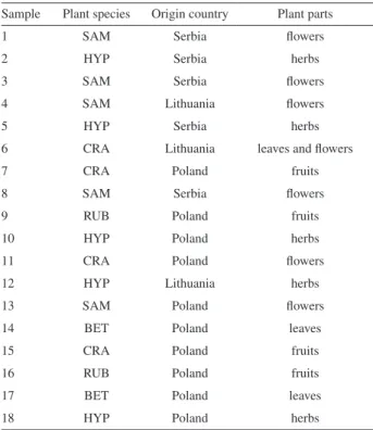
Eighteen samples of five herbal tea plant species from Lithuania (3 samples), Poland (10 samples) and Serbia (5 samples) were analyzed in this study (see details in Table 1). These samples represent 5 different species (Sambucus nigra L., Hypericum perforatum L.,
Crataegus oxyacantha auct. non L., Rubus idaeus L.and
Betula species L.), with the plant parts analyzed being flower, leaves with flowers, fruits, leaves and herbs.
In the mineralization process for further ICP OES determination of the analytes, dried and milled samples were mixed with 65% v/v HNO3 (Qhemis, Indaiatuba, SP, Brazil) and 30% v/v H2O2 (Synth, Diadema, SP, Brazil). The HNO3 had been previously purified by sub-boiling distillation using Distillacid™ BSB-939-IR (Berghof, Eningen, Germany). Multi-element standard solutions for the calibration curve were prepared from stock standard
solutions of 1000 mg L-1 (Fluka Analytical, Switzerland) by subsequent dilutions with 2% v/v HNO3. All volumetric flasks and glassware were washed, kept in 10% v/v HNO3 for 24 h, rinsed with deionized water and dried before use. Deionized water (resistivity > 18.2 MΩ cm) was generated using a Milli-Q® Plus Total Water System (Millipore Corp., Bedford, MA, USA).
Sample preparation and mineralization
All herbal samples were dried beforehand in an oven at 60 °C up to constant mass, milled using a multi-processor and sieved in order to obtain particle size lower than 500 µm.
A d i g e s t e r b l o c k w i t h P FA c l o s e d ve s s e l s (perfluoroalkoxy, Savillex, MN, USA) was employed for sample mineralization. PFA vessels of 50 mL were used and samples digested in triplicate according to the following procedure: 200 mg of tea material was accurately weighed in PFA vessels and kept overnight (approximately 16 h) with 2.0 mL of 65% v/v HNO3 at room temperature. One mL of 30% v/v H2O2 was added and the solution heated at 95 °C for 180 min. NIST 1515 (apple leaves), NIST 1573a (tomato leaves) and FO-01/2012 (Brachiaria Brizantha cv Marandu, EMBRAPA) reference materials were also digested for quality control of the measurements.
Table 1. Herbal tea samples description
Sample Plant species Origin country Plant parts
1 SAM Serbia flowers
2 HYP Serbia herbs
3 SAM Serbia flowers
4 SAM Lithuania flowers
5 HYP Serbia herbs
6 CRA Lithuania leaves and flowers
7 CRA Poland fruits
8 SAM Serbia flowers
9 RUB Poland fruits
10 HYP Poland herbs
11 CRA Poland flowers
12 HYP Lithuania herbs
13 SAM Poland flowers
14 BET Poland leaves
15 CRA Poland fruits
16 RUB Poland fruits
17 BET Poland leaves
18 HYP Poland herbs
After digestion, the PFA tubes were cooled, the digests filtered through filter paper (Unifil, Germany) to 15 mL volumetric flasks and the volume made up to 10 mL with high purity deionized water. The final solutions were analyzed by ICP OES (iCAP 6000, Thermo Scientific, Waltham, MA, USA).
Infusions
Infusions were prepared as follows: 200 mg of the sample were weighed into glass beakers. To this was added 10 mL of boiled deionized water, after which they were covered by watch glasses to extract sample components. After a twenty-minute extraction period, the tea infusion was filtered to 15 mL volumetric flasks, acidified with one drop of concentrated HNO3 (65% v/v) and the final volume adjusted to 10 mL with deionized water. Tea infusion solutions were also analyzed by ICP OES.
LIBS instrumentation
Experiments with LIBS were carried out with a Nd:YAG laser (Model J200, Applied Spectra, California, USA) which emits a laser pulse at 1064 nm (maximum energy of 100 mJ). The laser was operated by Axiom 2.5 software in a single laser pulse of 8 ns duration at a frequency of 10 Hz. This instrument is equipped with an ablation chamber with an HEPA air cleaner to remove ablated particles, as well as an automated XYZ stage and a 1280 × 1024 CMOS color camera imaging system. The
emission of the laser-induced plasma was collected using an optical fiber bundle coupled with a 6-channel CCD spectrometer covering wavelengths from 186 to 1042 nm (12288 variables).
LIBS analysis
The herbal samples (particle sizes lower than 500 µm) were weighed (approx. 400 mg) on analytical balances (model AY 220, Shimadzu, Kyoto, Japan) in order to facilitate LIBS analysis. The samples were pressed under 10 t inch-1 to form pellets with 12 mm in diameter. Pellets samples numbered 8, 12 and 16 (see Table 1 for details) were prepared in duplicate for preliminary studies using LIBS (optimization of the system). These plants belonged to the species Sambucus nigra (sample 8), Hypericum perforatum (sample 12) and Rubus idaeus (sample 16).
Doehlert design
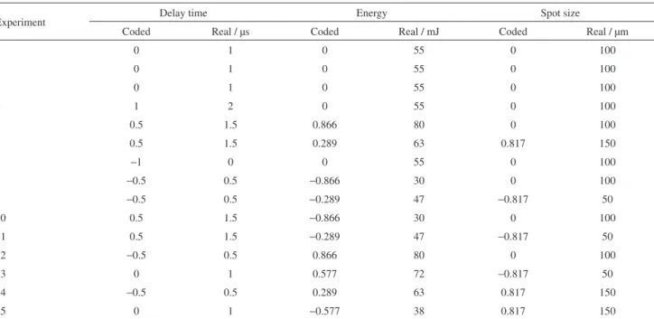
The additional instrumental parameters of the LIBS were evaluated through the use of Doehlert design.28 The variables chosen were delay time (0-2.0 µs, varied in 5 levels), laser energy (30-80 mJ, varied in 7 levels) and spot size (50-150 µm, varied in 3 levels). Table 2 shows the Doehlert experimental conditions. Spectral lines for Ca, K and Mg were monitored for regression model proposition in order to establish the commitment working condition for all analytes. Gate width of the measurements was 1.05 ms.
Table 2. Variables evaluated for LIBS and its levels (coded and real scale) in the Doehlert design
Experiment Delay time Energy Spot size
Coded Real / µs Coded Real / mJ Coded Real / µm
1 0 1 0 55 0 100
2 0 1 0 55 0 100
3 0 1 0 55 0 100
4 1 2 0 55 0 100
5 0.5 1.5 0.866 80 0 100
6 0.5 1.5 0.289 63 0.817 150
7 −1 0 0 55 0 100
8 −0.5 0.5 −0.866 30 0 100
9 −0.5 0.5 −0.289 47 −0.817 50
10 0.5 1.5 −0.866 30 0 100
11 0.5 1.5 −0.289 47 −0.817 50
12 −0.5 0.5 0.866 80 0 100
13 0 1 0.577 72 −0.817 50
14 −0.5 0.5 0.289 63 0.817 150
ICP OES analysis
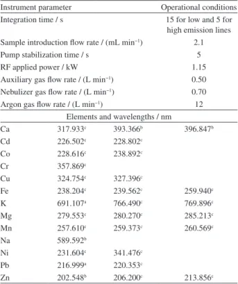
The aim of this study was to quantify by ICP OES macronutrients (Ca, K and Mg), micronutrients (Co, Cu, Fe, Mn, and Zn) and toxic elements (Cd, Cr, Ni and Pb) present in herbal plants in the form of digests and infusions. Table 3 shows the instrumental parameters and wavelengths chosen for each analyte. The ICP OES instrument used allows axial and radial views to be monitored sequentially.
Results and Discussion
ICP OES determinations
Three certified reference materials were analyzed in order to verify the accuracy of the method proposed and help in the wavelength and view modes selection. When the certified and obtained values were compared, the relative errors (%) for the macroelements (Ca, K, Mg and Na) ranged from 3 in the case of Mg to 24% in the case of Na (with an average of 8%). An unpaired t-test was calculated and the average t
calculated value was 2.22 (tabulated value with two degrees of freedom and 95% of confidence level = 4.303). In the case of microelements the relative errors calculated were: 12 (for Co), 3 (Cu), 32 (Fe), 12 (Mn) and 44% (Zn). For the toxic elements the relative errors were 12 (Cd), 40 (Cr), 25 (Ni)
and 25% (Pb). As can be observed, the relative errors for the micro and toxic elements were higher than those observed in the macroelements. This observation can be explained due to low elements concentration levels observed for micro and toxic elements. Actually, the concentrations of the macroelements are, in average, 300 times higher than those presented by the others.
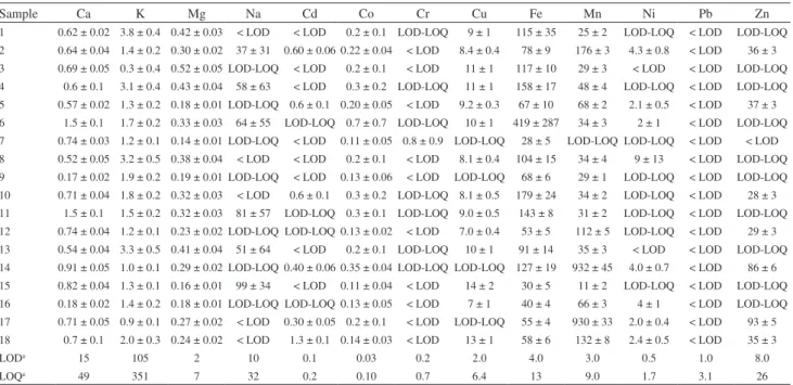
Table 4 shows the concentration of elements determined in the mineralized samples. Calcium, K and Mg concentrations were expressed in % (m/m) and the remainder in mg kg-1. The level of elements determined in this study by ICP OES is comparable to the results obtained by the same technique in other studies of the elemental composition of medicinal herbs and their infusions.3-5 In the case of infusions only Ca, K and Mg were observed in all samples. For the other analytes, in several cases, the concentrations were below the limits of detection (LOD) or quantification (LOQ) values.
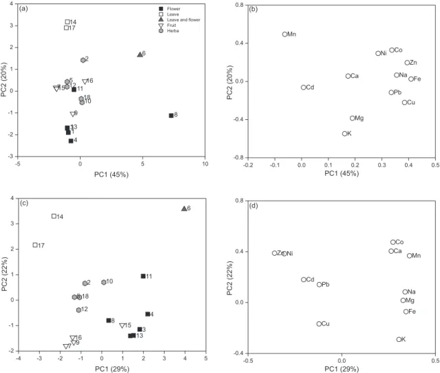
In order to obtain a global vision of all analytes and their relations, PCA was calculated separately using Pirouette 4.5 (Infometrix, Bothell, USA) for each type of data set (infusions and mineralized, Table 4) and the data set autoscaled. Figures 1a and 1b plot the scores (1a) and loadings (1b) for the infusions, but it proved difficult to observe a clear difference among the different types of samples and their characteristics (see Table 1 for further details). Some elements (see Figure 1b, loadings) are positively correlated (Co, Ni, Zn, Fe, Na, Pb and Cu).
However, several characteristic herbs can be depicted in Figure 1a. For example, two samples (samples 14 and 17) of Betulae folium originating in Poland are located in the upper left corner of plot PC1 vs. PC2. Two samples of
Crataegi fructus are also seen in the left-hand side of the plot (samples 7 and 15), and a group of herbs, mainly of the species Sambucus nigra (samples 1, 3, 4 and 13) in the lower left.
Figures 1c and 1d show the scores and loadings for mineralization, respectively. Analysis of the scores plot (Figure 1c) indicates a difference among types of teas: leaves (open squares) are related to Zn and Ni concentrations, leaves with flower (gray triangle) to Co, Ca and Mn concentrations and flower (black squares) to K, Na, Mg and Fe content. In Figure 1c tendencies generally similar to Figure 1a can be discerned. Again, two samples (14 and 17) of Betulae folium are far removed from the remainder in the upper left area of the plot. On the other hand, it is possible to detect a group of herbs in the lower right from the species Sambucus nigra (samples 1, 3, 4 and 13). After combined interpretation of the results shown in Figures 1a and 1c, it can be concluded that the herb samples analyzed belonged to specific plant species and Table 3. Instrumental parameters for ICP OES determinations
Instrument parameter Operational conditions Integration time / s 15 for low and 5 for
high emission lines Sample introduction flow rate / (mL min−1) 2.1
Pump stabilization time / s 5
RF applied power / kW 1.15
Auxiliary gas flow rate / (L min−1) 0.50 Nebulizer gas flow rate / (L min−1) 0.70 Argon gas flow rate / (L min−1) 12
Elements and wavelengths / nm
Ca 317.933c 393.366b 396.847b
Cd 226.502c 228.802c
Co 228.616c 238.892c
Cr 357.869c
Cu 324.754c 327.396c
Fe 238.204c 239.562c 259.940c
K 691.107a 766.490c 769.896c
Mg 279.553c 280.270c 285.213c
Mn 257.610c 259.373c 260.569c
Na 589.592b
Ni 231.604c 341.476c
Pb 216.999a 220.353c
Zn 202.548b 206.200c 213.856c
represented different morphological plant parts, with these two factors causing their characteristic distribution in the two-dimensional plots obtained by PCA. This conclusion confirms earlier studies of elemental concentrations in medicinal herbs obtained using the AAS technique.1,20-23
LIBS analysis
LIBS equipment parameters need to be optimized in order to obtain spectral signals with a high signal-to-background ratio (SBR). In this context, three parameters were evaluated using a Doehlert design (see Table 2) and the following atomic (I) emission lines were monitored (SBR, area and height): Ca I 527.027 nm, K I 693.878 and Mg I 517.268 nm. These lines were monitored in samples 8, 12 and 16 (representative samples, see Table 1).
For the experiments presented in Table 2, regression models were calculated for samples 8, 12 and 16 (1 model for each sample). In these models desirability function was calculated to cover SBR, signal area and height for Ca, K and Mg individually. Using this approach, each response was converted into numbers from 0 (undesired response, low SBR, area and height) to 1 (desired response, high SBR, area and height). After this, the individual desirability was combined into one single response (D, global desirability).29 Three models were calculated for global desirability (one for each sample type) and 10 coefficients were obtained: constant (b0), linear coefficients (b1, b2 and b3), quadratic coefficients (b11, b22 and b33) and interaction coefficients
(b12, b13 and b23). The significance of these coefficients was calculated using analysis of variance (ANOVA) table with 95% confidence level.
Figure 2 shows contour plots for sample 8 (Figure 2a) and 16 (Figure 2b). For sample 12 was not possible to obtain a significant model. A compromise condition for all types of samples was established with a delay time of 1.0 µs and energy of 70 mJ (see circle in Figures 2a and 2b). Spot size was not relevant to the range studied and was fixed at 100 µm. With this working condition, the predicted D values for samples 8 and 16 were 0.4 and 0.1, respectively. After testing commitment condition, obtained D values were 0.5 and 0.1 for samples 8 and 16, respectively, confirming a high level of concordance between both values.
This condition was tested for all 18 samples and the subsequent typical emission spectra are shown in Figure 3. Figure 3a (sample 6, leaves and flowers) shows strong emission lines for C, Ca, K, Mg, N and O (the symbols I and II represent atomic and emission lines, respectively). The same tendency was observed for the other samples: Figure 3b (sample 14, leaves), Figure 3c (sample 2, herbs), Figure 3d (sample 15, fruits) and Figure 3e (sample 13, flowers).
Calibration models (multivariate and univariate)
For Ca, Mg and K calibration models were calculated and two strategies tested: (i) multivariate using the whole signal profile (186 to 1042 nm, 12288 variables) and Table 4. Elements concentration (Ca, K and Mg in % m/m, the other elements in mg kg-1) for the mineralization (n = 3)
Sample Ca K Mg Na Cd Co Cr Cu Fe Mn Ni Pb Zn
1 0.62 ± 0.02 3.8 ± 0.4 0.42 ± 0.03 < LOD < LOD 0.2 ± 0.1 LOD-LOQ 9 ± 1 115 ± 35 25 ± 2 LOD-LOQ < LOD LOD-LOQ 2 0.64 ± 0.04 1.4 ± 0.2 0.30 ± 0.02 37 ± 31 0.60 ± 0.06 0.22 ± 0.04 < LOD 8.4 ± 0.4 78 ± 9 176 ± 3 4.3 ± 0.8 < LOD 36 ± 3 3 0.69 ± 0.05 0.3 ± 0.4 0.52 ± 0.05 LOD-LOQ < LOD 0.2 ± 0.1 < LOD 11 ± 1 117 ± 10 29 ± 3 < LOD < LOD LOD-LOQ 4 0.6 ± 0.1 3.1 ± 0.4 0.43 ± 0.04 58 ± 63 < LOD 0.3 ± 0.2 LOD-LOQ 11 ± 1 158 ± 17 48 ± 4 LOD-LOQ < LOD LOD-LOQ 5 0.57 ± 0.02 1.3 ± 0.2 0.18 ± 0.01 LOD-LOQ 0.6 ± 0.1 0.20 ± 0.05 < LOD 9.2 ± 0.3 67 ± 10 68 ± 2 2.1 ± 0.5 < LOD 37 ± 3 6 1.5 ± 0.1 1.7 ± 0.2 0.33 ± 0.03 64 ± 55 LOD-LOQ 0.7 ± 0.7 LOD-LOQ 10 ± 1 419 ± 287 34 ± 3 2 ± 1 < LOD LOD-LOQ 7 0.74 ± 0.03 1.2 ± 0.1 0.14 ± 0.01 LOD-LOQ < LOD 0.11 ± 0.05 0.8 ± 0.9 LOD-LOQ 28 ± 5 LOD-LOQ LOD-LOQ < LOD < LOD 8 0.52 ± 0.05 3.2 ± 0.5 0.38 ± 0.04 < LOD < LOD 0.2 ± 0.1 < LOD 8.1 ± 0.4 104 ± 15 34 ± 4 9 ± 13 < LOD LOD-LOQ 9 0.17 ± 0.02 1.9 ± 0.2 0.19 ± 0.01 LOD-LOQ < LOD 0.13 ± 0.06 < LOD LOD-LOQ 68 ± 6 29 ± 1 LOD-LOQ < LOD LOD-LOQ 10 0.71 ± 0.04 1.8 ± 0.2 0.32 ± 0.03 < LOD 0.6 ± 0.1 0.3 ± 0.2 LOD-LOQ 8.1 ± 0.5 179 ± 24 34 ± 2 LOD-LOQ < LOD 28 ± 3 11 1.5 ± 0.1 1.5 ± 0.2 0.32 ± 0.03 81 ± 57 LOD-LOQ 0.3 ± 0.1 LOD-LOQ 9.0 ± 0.5 143 ± 8 31 ± 2 LOD-LOQ < LOD LOD-LOQ 12 0.74 ± 0.04 1.2 ± 0.1 0.23 ± 0.02 LOD-LOQ LOD-LOQ 0.13 ± 0.02 < LOD 7.0 ± 0.4 53 ± 5 112 ± 5 LOD-LOQ < LOD 29 ± 3 13 0.54 ± 0.04 3.3 ± 0.5 0.41 ± 0.04 51 ± 64 < LOD 0.2 ± 0.1 LOD-LOQ 10 ± 1 91 ± 14 35 ± 3 < LOD < LOD LOD-LOQ 14 0.91 ± 0.05 1.0 ± 0.1 0.29 ± 0.02 LOD-LOQ 0.40 ± 0.06 0.35 ± 0.04 LOD-LOQ LOD-LOQ 127 ± 19 932 ± 45 4.0 ± 0.7 < LOD 86 ± 6 15 0.82 ± 0.04 1.3 ± 0.1 0.16 ± 0.01 99 ± 34 < LOD 0.11 ± 0.04 < LOD 14 ± 2 30 ± 5 11 ± 2 LOD-LOQ < LOD LOD-LOQ 16 0.18 ± 0.02 1.4 ± 0.2 0.18 ± 0.01 LOD-LOQ LOD-LOQ 0.13 ± 0.05 < LOD 7 ± 1 40 ± 4 66 ± 3 4 ± 1 < LOD LOD-LOQ 17 0.71 ± 0.05 0.9 ± 0.1 0.27 ± 0.02 < LOD 0.30 ± 0.05 0.2 ± 0.1 < LOD LOD-LOQ 55 ± 4 930 ± 33 2.0 ± 0.4 < LOD 93 ± 5 18 0.7 ± 0.1 2.0 ± 0.3 0.24 ± 0.02 < LOD 1.3 ± 0.1 0.14 ± 0.03 < LOD 13 ± 1 58 ± 6 132 ± 8 2.4 ± 0.5 < LOD 35 ± 3
LODa 15 105 2 10 0.1 0.03 0.2 2.0 4.0 3.0 0.5 1.0 8.0
LOQa 49 351 7 32 0.2 0.10 0.7 6.4 13 9.0 1.7 3.1 26
Figure 1. Scores and loadings plots for the datasets obtained for (a and b) infusion and (c and d) mineralization.
Figure 2. Contour plots obtained for the models after LIBS parameters optimization for samples (a) 8 and (b) 16. The circle represents the optimum condition.
(ii) univariate. In this instance, the goal was to propose an expeditious method for direct determination of these three macronutrients in solid samples.
In the case of univariate calibration, the signals depicted in Figure 4 were used. In both strategies (multivariate or
and sum after normalization by C signals (I 193.090 and I 247.856 nm).30
For Ca and Mg the best results (lower prediction error) were obtained with signal normalized by maximum and by norm, respectively. In order to evaluate the quality of the proposed models standard error of cross-validation (SECV),
calculated using the calibration data set (14 samples) and tested in 4 samples (validation data set).
For LOD and LOQ calculation using univariate calibration, the standard deviation was obtained using signal noise in the surrounding wavelengths near Ca, K and Mg signals (see Figure 4).32 Table 5 shows the parameters
for the models and Figure 5 reference (obtained by ICP OES) and predicted concentrations for Ca (Figure 5a), K (Figure 5b) and Mg (Figure 5c). The univariate models
Figure 4. Emission lines selected for (a) Ca; (b) K and (c) Mg to calculate the univariate regression models.
using signal area (Ca) and height (K and Mg) presented error values lower than the multivariate calibration models.
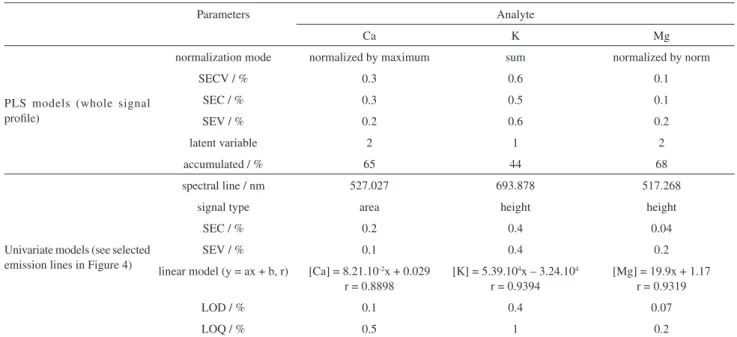
For Ca, the best results were obtained after data set normalization by the maximum of each spectrum. SEC values for PLS and univariate models (signal area) were 0.3 and 0.2%, respectively, and the LOD obtained was 0.1%. Reference and predicted concentration for univariate models (Figure 5a) showed a strong correlation at r = 0.8898. In the case of K, the best results were obtained after the sum of the signals. Error values ranged from 0.4 (SEC for univariate using signal height) to 0.6% (SEV using whole signal profile). LOD value was 0.4%. Magnesium, while presenting the highest relative intensity among the analytes studied, simultaneously presented the lowest LOD values (0.07%) and the best normalization model was normalization by individual norm. The correlation between the reference and predicted values was 0.9319 for univariate model (see Figure 5c).
Conclusions
The results obtained confirm that chemometric methods could be introduced to effectively extract spectral data, samples classification (PCA) and to solve multivariate problems like parameter optimization and multivariate simultaneous analysis (PLS). With the benefit of applying LIBS for the monitoring of multiple elements in medicinal herbs, PLS was combined with LIBS as a multivariate calibration method and a set of univariate models
developed (Table 5). These models successfully predict high concentrations of Ca, Mg and K with high correlation coefficient and low SEC and LOD for univariate models.
It can be also inferred that the combination of LIBS, ICP OES and chemometric tools has significant potential for the development and implementation of methods towards exploring concentrations of essential and toxic elements in medicinal herbs.
Acknowledgments
This project was supported by the Ministry of Science and Higher Education of the Republic of Poland, from the subsidy for Quality Promotion, under the Leading National Research Centre (KNOW) program for the years 2012-2017. The authors are also grateful to the Conselho Nacional de Desenvolvimento Científico e Tecnológico (CNPq, process 401074/2014-5), Empresa Brasileira de Pesquisa Agropecuária (EMBRAPA), Coordenação de Aperfeiçoamento de Pessoal de Nível Superior (CAPES) and Analitica Thermo for the loan of ICP OES instrument.
References
1. Arceusz, A.; Radecka, I.; Wesolowski, M.; Food Chem. 2010, 120, 52.
2. Gogoasa, I.; Jurca, V.; Alda, L. M.; Velciov, A.; Rada, M.; Alda, S.; Sirbulescu, C.; Bordean, D. M.; Gergen, I.; J. Hortic. For. Biotechnol. 2013, 17, 65.
Table 5. Regression models (multivariate and univariate) parameters for the models calculated for Ca, K and Mg
Parameters Analyte
Ca K Mg
PLS models (whole signal profile)
normalization mode normalized by maximum sum normalized by norm
SECV / % 0.3 0.6 0.1
SEC / % 0.3 0.5 0.1
SEV / % 0.2 0.6 0.2
latent variable 2 1 2
accumulated / % 65 44 68
Univariate models (see selected emission lines in Figure 4)
spectral line / nm 527.027 693.878 517.268
signal type area height height
SEC / % 0.2 0.4 0.04
SEV / % 0.1 0.4 0.2
linear model (y = ax + b, r) [Ca] = 8.21.10-2x + 0.029 r = 0.8898
[K] = 5.39.104x – 3.24.104 r = 0.9394
[Mg] = 19.9x + 1.17 r = 0.9319
LOD / % 0.1 0.4 0.07
LOQ / % 0.5 1 0.2
3. Pytlakowska, K.; Kita, A.; Janoska, P.; Polowniak, M.; Kozik, V.; Food Chem. 2012, 135, 494.
4. Basgel, S.; Erdemoglu, S. B.; Sci. Total Environ. 2006, 359, 82. 5. Karadas, C.; Kara, D.; Food Chem. 2012, 130, 196.
6. Sing, V.; Garg, A. N.; Appl. Radiat. Isot. 1997, 48, 97. 7. Kumar, A.; Nair, A. G. C.; Reddy, A. V. R.; Garg, A. N.; J.
Pharm. Biomed. Anal. 2005, 37, 631.
8. Pasquini, C.; Cortez, J.; Silva, L. M. C.; Gonzaga, F. B.; J. Braz. Chem. Soc. 2007, 18, 463.
9. Rai, P. K.; Srivastava, A. K.; Sharma, B.; Preeti, D.; Mishra, A. K.; Watal, G.; Evidence-Based Complementary Altern. Med.
2013, 2013, ID 406365. DOI: 10.1155/2013/406365.
10. Liu, X.; Zhang, Q.; Wu, Z.; Shi, X.; Zhao, N.; Qiao, Y.; Sensors
2015, 15, 642.
11. Barbier, S.; Perrier, S.; Freyermuth, P.; Perrin, D.; Gallard, B.; Gilon, N.; Spectrochim. Acta, Part B 2013, 88, 167.
12. Aquino, F. W. B.; Pereira-Filho, E. R.; Talanta 2015, 134, 65. 13. Carvalho, R. R. V.; Coelho, J. A. O.; Santos, J. M.; Aquino, F.
W. B.; Carneiro, R. L.; Pereira-Filho, E. R.; Talanta 2015, 134, 278.
14. Aquino, F. W. B.; Santos, J. M.; Carvalho, R. R. V.; Coelho, J. A. O.; Pereira-Filho, E. R.; RSC Adv. 2015, 5, 67001. 15. Bousquet, B.; Travaillé, G.; Ismael, A.; Canioni, L.; Pierres, K.
M.; Brasseur, E.; Roy, S.; HechoI, Il.; Larregieu, M.; Tellier, S.; Potin-Gautier, M.; Boriachon, T.; Wazen, P.; Diard, A.; Belbeze, S.; Spectrochim. Acta, Part B 2008, 63, 1085.
16. Gondal, M. A.; Seddigi, Z. S.; Nasr, M. M.; Gondal, B.; J. Hazard. Mater. 2010, 175, 726.
17. Andersen, M. S.; Frydenvang, J.; Henckel, P.; Rinnan, A.; Food Control 2016, 64, 226.
18. Cremers, D. A.; Chinni, R. C.; Appl. Spectrosc. Rev. 2009, 44, 457.
19. Galbács, G.; Anal. Bioanal. Chem. 2015, 407, 7537.
20. Lemberkovics, E.; Czinner, E.; Szentmihalyi, K.; Balazs, A.; Szoke, E.; Food Chem. 2002, 78, 119.
21. Razic, S.; Dogo, S.; Slavkovic, L.; Popovic, A.; J. Serb. Chem. Soc. 2005, 70, 1347.
22. Konieczynski, P.; Arceusz, A.; Wesolowski, M.; Biol. Trace Elem. Res. 2016, 170, 466.
23. Konieczynski, P.; Cent. Eur. J. Chem. 2013, 11, 519. 24. Yang, J.; Chen, L. H.; Zhang, Q.; Lai, M. X.; Wang, Q.; J. Sep.
Sci. 2007, 30, 1276.
25. Tian, R.; Xie, P.; Liu, J.; J. Chromatogr. A 2009, 1216, 2150. 26. Martins, R. C.; Lopes, V. V.; Valentão, P.; Carvalho, J. C.;
Amaral, M. T.; Batista, M. T.; Andrade, P. B.; Silva, B. M.; Nat. Prod. Res. 2008, 22, 1560.
27. Gok, S.; Severcan, M.; Goormaghtigh, E.; Kandemir, I.; Severcan, F.; Food Chem. 2015, 170, 234.
28. Ferreira, S. L. C.; Santos, W. N. L.; Quintella, C. M.; Barros Neto, B.; Bosque-Sendra, J. M.; Talanta 2004, 64, 1061. 29. Derringer, G.; Suich, R.; J. Qual. Technol. 1980, 12, 214. 30. Castro, J. P.; Pereira-Filho, E. R.; J. Anal. At. Spectrom. 2016,
DOI 10.1039/c6ja00224b.
31. Santos, P. M.; Wentzell, P. D.; Pereira-Filho, E. R.; Food Anal. Methods 2012, 5, 89.
32. Pereira, F. M. V.; Pereira-Filho, E. R.; Bueno, M. I. M. S.; J. Agric. Food Chem. 2006, 54, 5723.
Submitted: June 24, 2016
Published online: August 16, 2016